Lecture08

\makecscover

来源审计与问题边界：什么叫 Mechanistic Interpretability

本讲追问一个比“模型是否答对”更困难的问题：给定一组已经训练好的参数，能否把模型内部计算反编译成人类可以检查的算法？Chris Olah 将这种工作称为 \term{mechanistic interpretability}（机制可解释性）。它并不满足于展示相关 activation 或生成自然语言理由，而是希望说明某组 weights、features 与 attention heads 如何组成一个可复现的计算过程。

本次重写以官方视频 pC4zRb_5noQ 为影音基准。Stanford CS25 V1 课程表把讲座列在 2021-11-15；课堂中 Olah 多次称 induction-head 结果尚未发表。后来文章在 2022-03-08 公开，Stanford Online 到 2022-07-17 才上传录像。讲义因此将课堂中的 tentative hypothesis、后来文章的补充证据与本讲的工程解释明确分层，不能用后见之明把每个说法写成定论。

视频没有公开独立 slide PDF。我们从官方 1080p 录像中恢复 64 张教学页，保留公式推导的独立步骤与最终 progressive state，省略重复曲线、空白转场、片尾，以及 50--55 分钟低清 Lexoscope live demo 的中间界面；demo 中的 cross-lingual/soft-induction 口头解释仍完整进入正文。

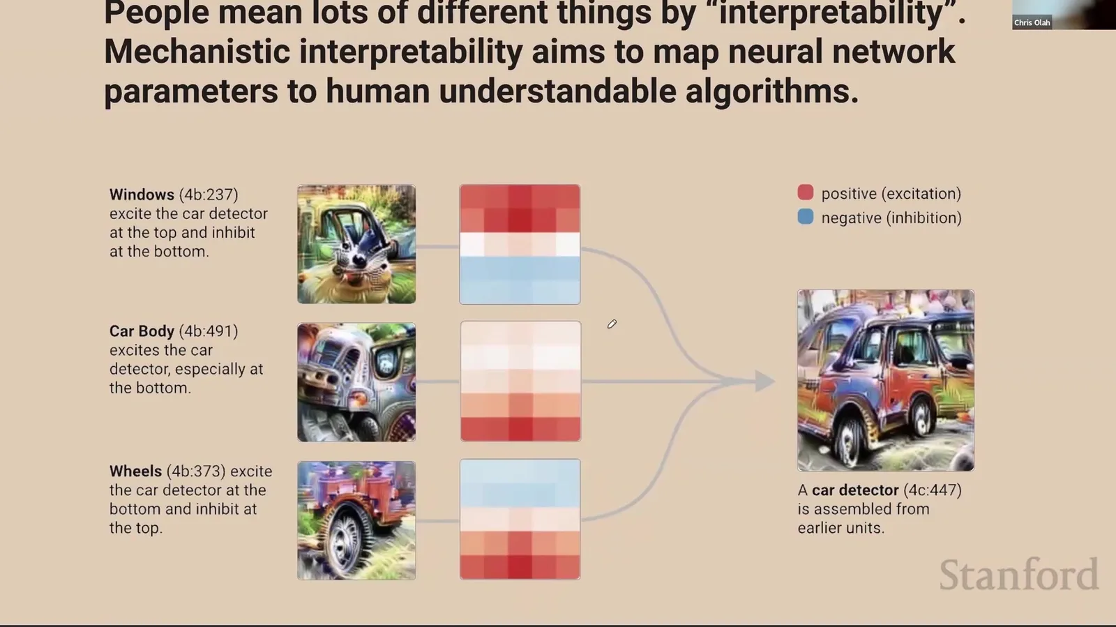
\lecturefigure{slide-01-interpretability-definition.jpg}{Mechanistic interpretability：把 neural-network parameters 映射回人类可理解的 algorithms。}{Stanford Online 官方视频 00:00:30--00:03:27。}

图左的 vision circuit 给出最小例子：wheel feature 喜欢图像底部的轮子、不喜欢顶部的轮子；window feature 具有相反的空间偏好；它们共同支持 car feature。重点不是“发现一个会叫 car 的 neuron”，而是看到 features 之间有方向、符号与位置关系，可以被解释成一段组合算法。

\teachervoice{Olah 的类比是：weights 像 compiled computer program，features/neurons 像 variables 或 registers。机制解释的任务是 reverse engineering，而不是为输出写一段听起来合理的事后故事。}

Interpretability 不是一个单一问题

层次	典型问题	本讲是否重点处理
Behavioral evaluation	模型在什么输入上成功或失败？	用来发现 ICL phase change，但不是终点。
Feature attribution	哪些 token/activation 与输出相关？	提供线索，单独不能证明 circuit。
Mechanistic analysis	参数怎样实现可执行算法？	本讲核心：QK/OV、path composition、induction。
Causal validation	移除组件后，目标行为会变化吗？	small-model ablation 是关键证据。
System/social explanation	数据、部署、人与制度如何共同产生结果？	超出本讲电路范围，不能由 circuits 自动回答。

为什么要做这种逆向工程

Olah 给出两类动机。科学动机是：人类不会手写一个能完成 ImageNet classification 或 GPT-3 behavior 的明确程序，但 gradient descent 能在参数中找到某种解；理解这个解可能发现新算法。安全动机是：如果系统被用于高影响场景，我们希望在 failure mode 被实际触发之前，识别参数中潜伏的“unknown unknowns”。

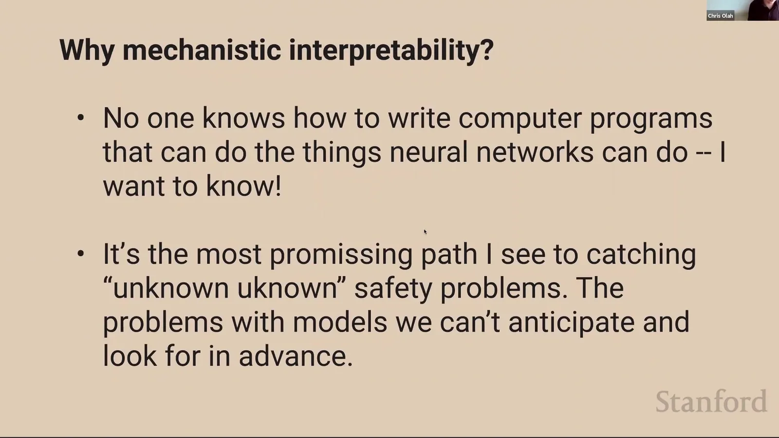
\lecturefigure{slide-02-why-mechanistic-interpretability.jpg}{为什么研究机制解释：发现 gradient descent 写出的算法，并提前识别未知失败模式。}{Stanford Online 官方视频 00:03:28--00:04:23。}

能解释一个 circuit，不等于解释整个模型

局部电路可以在特定模型、特定 prompt family 和特定 metric 上被验证；它不自动覆盖 MLP、训练数据、其他 heads、分布外行为或社会部署后果。Mechanistic interpretability 的价值来自可检验的局部进展，而不是提前宣称“模型已经透明”。

课堂当时的证据强度

这堂课的特殊之处在于讲者主动展示研究的未完成状态。他此前主要研究 vision ConvNets，把同样方法迁移到 language models 仍属新工作；因此我们需要保留“这是 hypothesis”“large model 目前只有 correlation”“可能有其他 mechanism”这些限定语。

\lecturefigure{slide-03-language-models-new-territory.jpg}{讲者的版本声明：语言模型机制解释仍很新，离成熟发表与完整解释有距离。}{Stanford Online 官方视频 00:04:24--00:05:39。}

\teachervoice{Olah 欢迎听众提出最基础的问题，也欢迎指出不清楚和错误之处。这个课堂语气非常重要：后面的 induction-head story 是一条有多种证据支持的研究路线，不是对所有 Transformer in-context learning 的最终封闭解释。}

本章小结

Mechanistic interpretability 把模型视为被 gradient descent 编译的程序，并尝试恢复其中的算法。它既服务于科学发现，也可能帮助安全审计，但必须区分局部 circuit、整体模型与部署系统，并严格记录每条结论的证据强度。

行为谜题：怎样量化 In-Context Learning

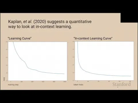
在研究内部电路前，首先要定义待解释的外部现象。\term{In-context learning}（ICL）指参数固定时，模型仅凭当前 context 中的 examples、pattern 或 instructions 改善后续预测。它看起来像模型在 prompt 内又执行了一次临时学习，因此成为大型语言模型最引人注意的能力之一。

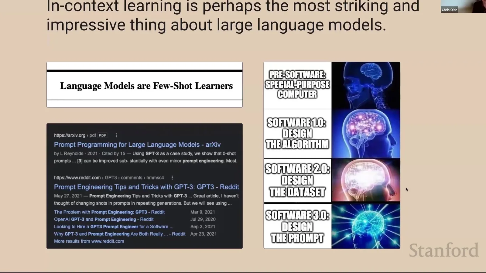
\lecturefigure{slide-04-in-context-learning-motivation.jpg}{In-context learning：固定参数的语言模型从 prompt/context 中临时获得新能力。}{Stanford Online 官方视频 00:05:40--00:06:51。}

\teachervoice{讲者把 ICL 称为大型语言模型最 striking 的性质之一，但这里的“learning”不是 gradient update。模型参数保持不变，变化发生在 residual activations 与 attention computation 中。}

两个 learning axis

普通 learning curve 以训练进度为横轴，观察模型随着 gradient steps 增加而改善；ICL curve 则固定某个 training snapshot，以 context token index 为横轴，观察同一 forward 中越靠后的 token 是否预测得更好。把两者放在一起，得到二维函数

\[ \mathcal{L}(s,i) =\mathbb{E}_{x}\left[-\log p_{\theta_s}(x_i\mid x_{<i})\right], \]

其中：

\(s\)：training snapshot 或累计训练 tokens；
\(i\)：当前 sequence 中的 token index；
\(\theta_s\)：snapshot \(s\) 的参数；
\(\mathcal{L}(s,i)\)：该 snapshot 在第 \(i\) 个 context position 的平均 next-token loss。

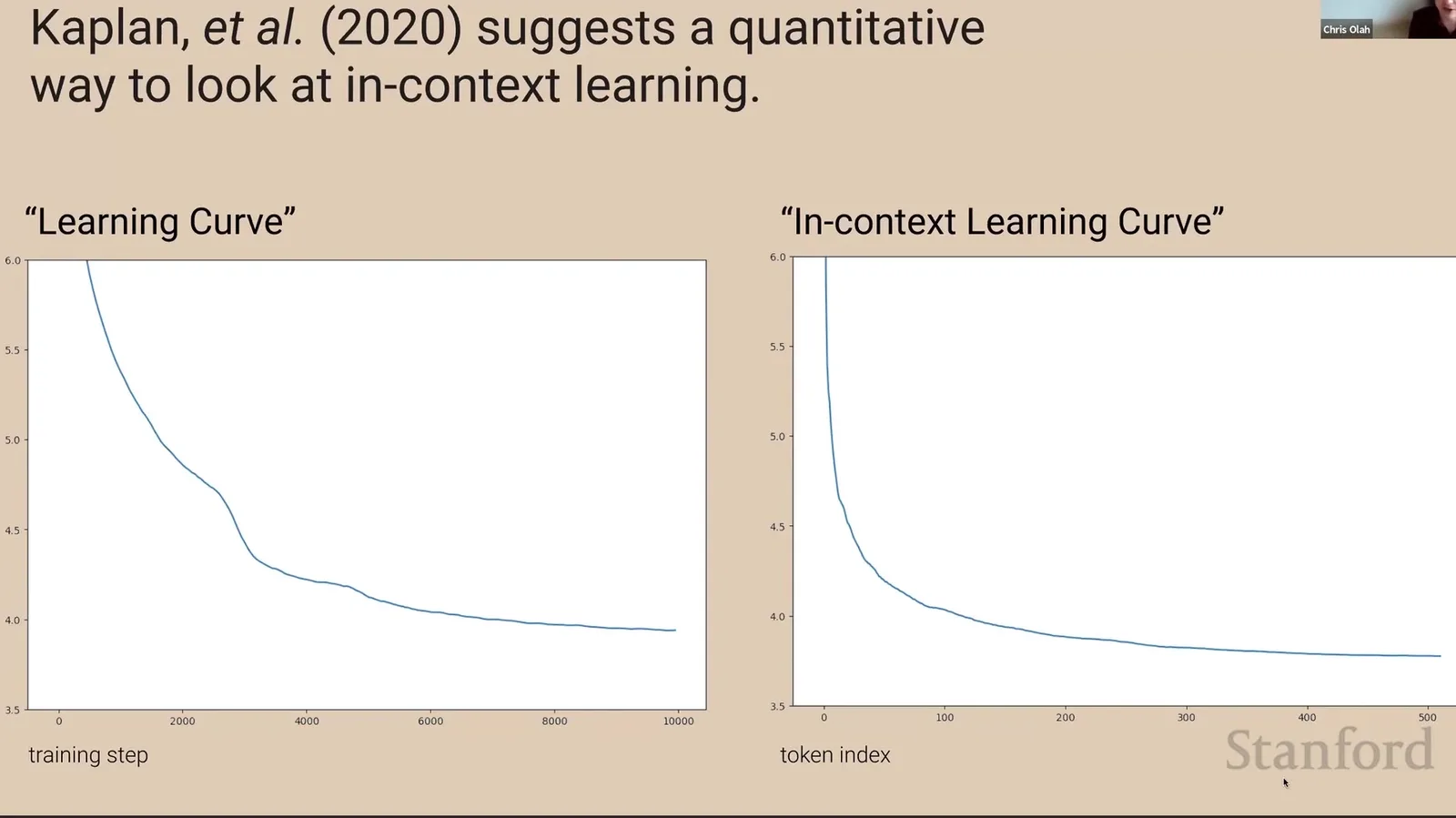
\lecturefigure{slide-05-learning-vs-in-context-curves.jpg}{Learning curve 与 in-context learning curve：训练时间轴和 context 位置轴。}{Stanford Online 官方视频 00:06:52--00:10:33。}

两种“学习”不能混为一谈

Training learning 改变 \(\theta_s\)；in-context learning 固定 \(\theta_s\)，只改变输入 prefix 和内部 activations。前者回答“模型训练得更久会怎样”，后者回答“同一模型看到更多 context 会怎样”。

二维 loss map 与 ICL score

把每个 snapshot 的 per-token loss 叠起来，纵轴为 context position、横轴为 snapshot，就得到二维地图。横切片是某个 token position 的 training curve；纵切片是某个 snapshot 的 ICL curve。讲者使用一个简单 summary statistic：

\[ S_{\mathrm{ICL}}(s) =\mathcal{L}(s,500)-\mathcal{L}(s,50). \]

若 \(S_{\mathrm{ICL}}<0\)，第 500 个 token 比第 50 个 token 更容易预测；
数值越负，late-context advantage 越强；
该指标只压缩 context-position improvement，不等价于 few-shot task accuracy；
token 50 与 500 是论文设置中的 operational choice，不是 ICL 的唯一合法定义。

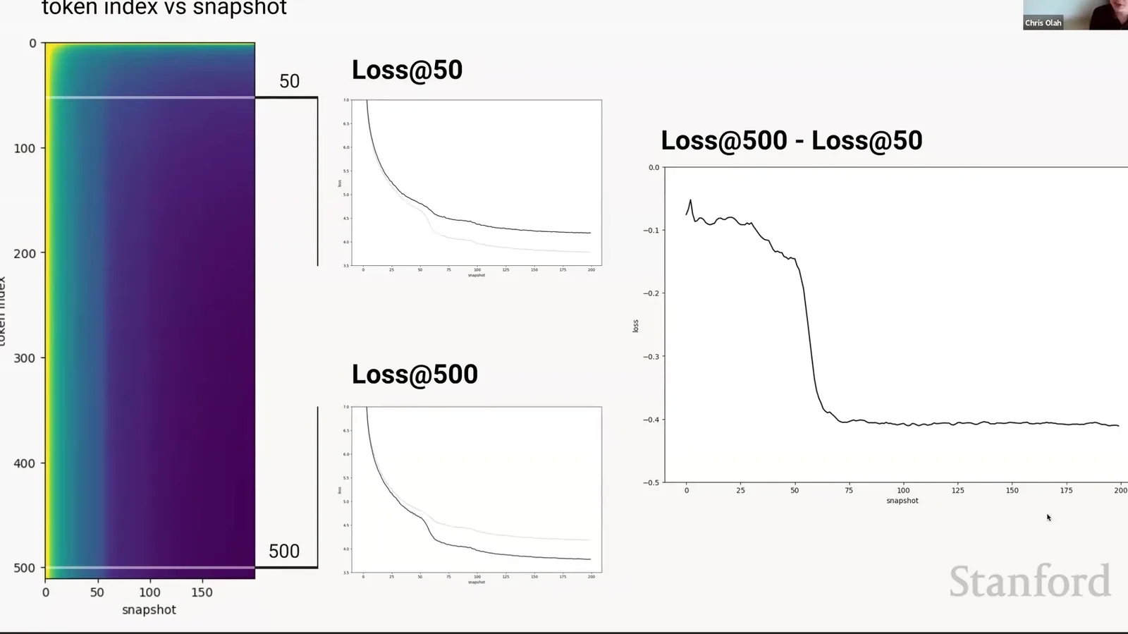
\lecturefigure{slide-06-token-snapshot-loss-map.jpg}{统一诊断图：token index × training snapshot loss，以及 \(\mathrm{Loss@500}-\mathrm{Loss@50}\)。}{Stanford Online 官方视频 00:10:34--00:12:45。}

读图：先看轴，再看右侧差分曲线

左侧热图显示每个 training snapshot 在不同 token index 上的 loss；中间的 Loss@50 与 Loss@500 是两条横切片；右侧差分曲线消去整体训练改善，突出“后半段 context 是否突然变得更有用”。

从 per-token loss 计算 ICL score 与 phase-change diagnostic。

def in_context_learning_score(loss_by_snapshot_and_token):
    loss_50 = loss_by_snapshot_and_token[:, 49]
    loss_500 = loss_by_snapshot_and_token[:, 499]
    score = loss_500 - loss_50  # more negative means stronger ICL
    slope = derivative(score, with_respect_to="log_training_tokens")
    return score, slope

0.4 nats 到底有多大

Negative log-likelihood 使用 natural logarithm 时单位为 nat。要换成 bits，除以 \(\ln 2\)：

\[ 0.4\ \mathrm{nats} =\frac{0.4}{\ln 2}\ \mathrm{bits} \approx 0.577\ \mathrm{bits/token}. \]

换句话说，模型对 late-context token 的 uncertainty 每 token 大约少半个 bit，粗略相当于每两 token 少一个 binary choice。这不是“准确率提高 40%”，也不能跨数据集直接比较，却足以说明 context 内新增信息被稳定利用。

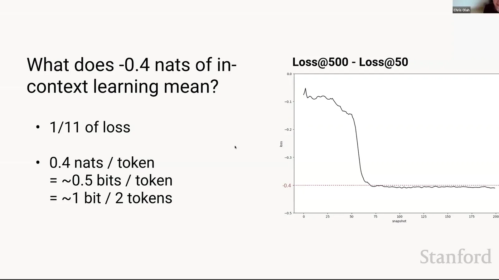
\lecturefigure{slide-07-meaning-of-point-four-nats.jpg}{效果量直觉：\(0.4\) nats 约为 \(0.5\) bits/token。}{Stanford Online 官方视频 00:12:46--00:13:47。}

\teachervoice{Olah 主动把 nats 转成 bits，是为了防止曲线上的小数被低估。Language modeling 每个 token 都累积损失，半个 bit/token 在长序列上会形成很大的 total log-likelihood difference。}

本章小结

ICL 的行为指标来自二维 loss surface：一个轴是训练进度，一个轴是 context position。\(\mathrm{Loss@500}-\mathrm{Loss@50}\) 把 late-token advantage 压缩为一条曲线，为后续寻找内部 circuit 提供了可干预的目标量。

Phase Change：从 loss bump 提出 circuit hypothesis

二维 loss map 的关键发现不是 ICL 缓慢增强，而是在很窄的训练窗口内突然出现。为了突出这种变化，研究者对 token-position curve 与 training trajectory 做差分/导数；热图中出现清晰竖线，普通 loss curve 也出现一个小 bump。

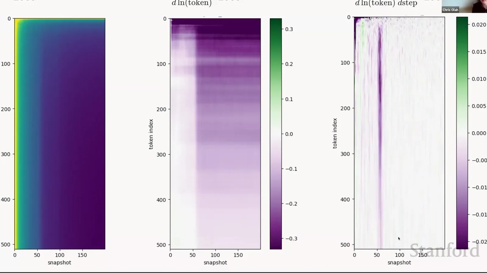
\lecturefigure{slide-08-per-step-learning-heatmaps.jpg}{Loss surface 与导数视图：窄训练窗口内出现明显结构变化。}{Stanford Online 官方视频 00:13:48--00:14:01。}

可把诊断量抽象写为

\[ D_i(s,i)=\frac{\partial \mathcal{L}(s,i)}{\partial \log i}, \qquad D_s(s)=\frac{\partial S_{\mathrm{ICL}}(s)}{\partial \log s}. \]

\(D_i\) 衡量增加相对 context 长度带来的 loss reduction；
\(D_s\) 衡量 ICL score 在训练中的变化速度；
narrow spike 表明行为在少量训练 steps 内快速改变；
导数放大噪声，因此必须对照原始 loss、多个 seeds 与多个 model sizes。

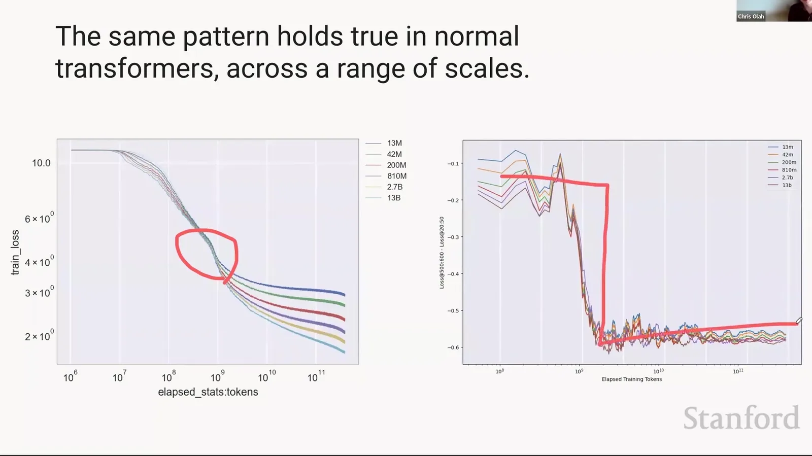
\lecturefigure{slide-09-phase-change-across-scales.jpg}{不同 model scales 中都能看到 loss bump 与 ICL 快速上升。}{Stanford Online 官方视频 00:14:02--00:15:11。}

“Phase change” 是经验描述，不是已证明的物理相变

曲线在有限 snapshots 中快速变化，并不证明 optimization trajectory 数学不连续。更稳妥的结论是：存在一个 narrow training interval，模型行为与内部 signatures 同时快速重组，值得提出机制假说并做干预。

从行为变化到内部机制

如果外部 ICL 在几百 steps 内突然增强，一个自然假设是模型内部也形成了新 circuit。要验证它，不能只继续看 loss；需要把参数分解为可解释 path，并比较一层与两层 attention-only models，因为前者没有该 phase change，后者有。

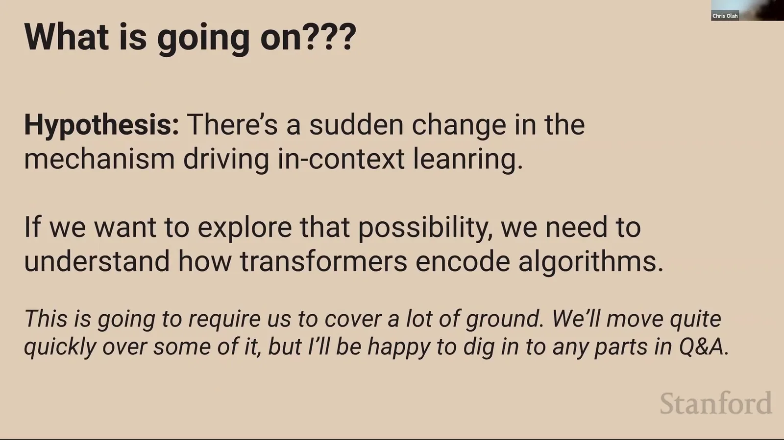
\lecturefigure{slide-10-sudden-mechanism-change-hypothesis.jpg}{研究假设：ICL 行为相变对应内部算法/电路的突然形成。}{Stanford Online 官方视频 00:15:12--00:15:31。}

\teachervoice{讲者用的是 “natural hypothesis”，不是 proof。行为 bump 只是搜索入口；只有当候选 circuit 在时间上出现、在结构上能实现目标算法、并且 ablation 会移除行为时，机制解释才逐渐成立。}

证据阶梯

后文会反复使用四种证据。为了避免混淆，先给出强度排序：

证据	例子	能支持什么
Representational plausibility	QK/OV 矩阵能实现 match 与 copy	说明 circuit 有能力，不证明实际被使用。
Temporal co-occurrence	Induction signature 与 ICL 同时出现	提供相关证据，可能有共同原因。
Behavioral generality	Copy、translation、pattern matching	说明机制不局限于单一 toy string。
Causal intervention	Ablate head 后 ICL score 回退	直接支持该组件对该 metric 的因果贡献。
Near-complete accounting	少量 paths 解释 toy model 主要 loss	在限定模型中接近完整，但不自动外推大型 LLM。

本讲中的证据类型与可支持结论。

本章小结

Phase change 把一个模糊的“模型似乎会从 context 学习”转成具体研究目标：解释窄窗口内的 ICL score 变化。行为曲线产生 hypothesis，真正的机制结论还需要 algebra、结构可行性、跨例泛化与 causal ablation。

一层 Attention-Only Transformer：先把模型化成可加路径

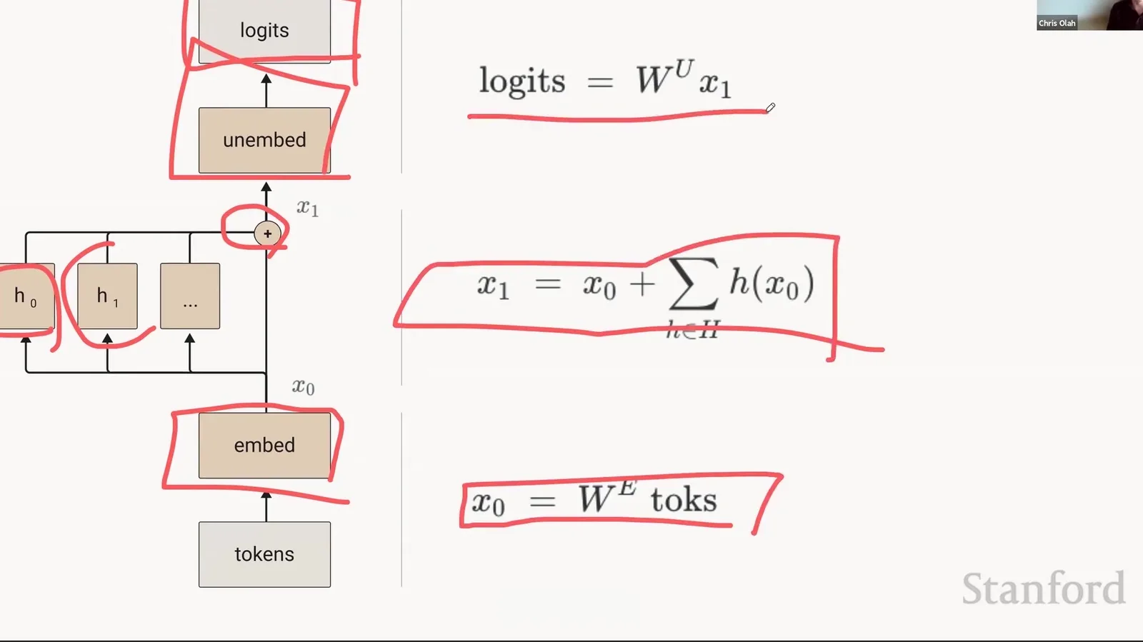
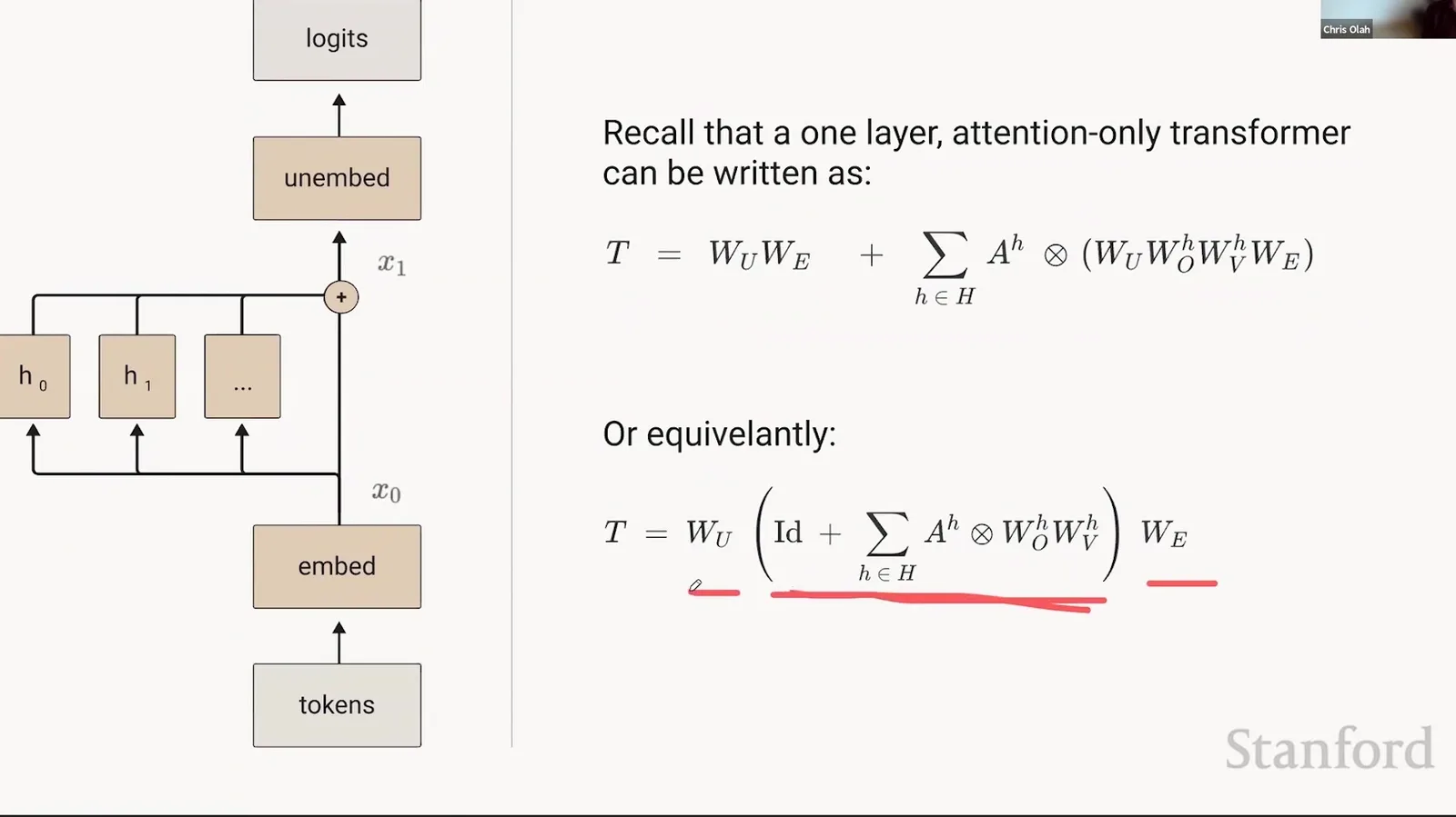
为得到精确代数，Olah 暂时移除 MLP、LayerNorm 与 bias，只保留一层 multi-head attention、residual connection、token embedding 与 unembedding。这不是现代 LLM 的完整架构，而是一个实验台：如果连这个系统都不能分解，就更难解释大型模型。

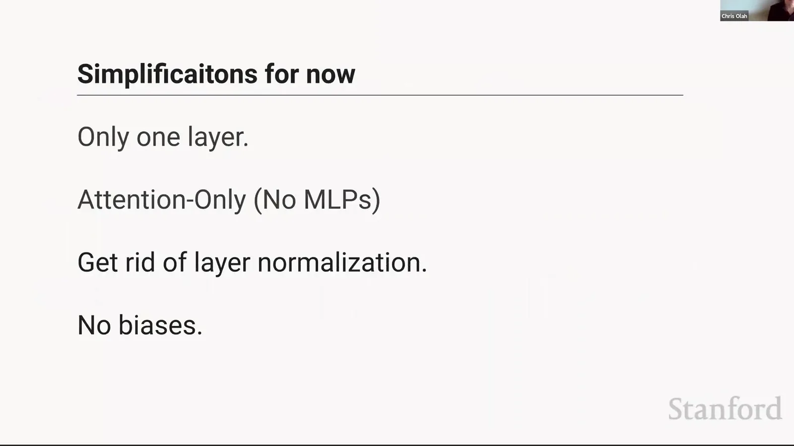
\lecturefigure{slide-11-one-layer-simplifications.jpg}{分析假设：one layer、attention-only、无 LayerNorm、无 bias。}{Stanford Online 官方视频 00:15:32--00:15:59。}

Toy model 的作用与边界

简化模型允许把每个 path 写成矩阵乘法并做近乎完整 accounting。它能发现 reusable concept，但不能证明相同公式在带 MLP、RMSNorm、RoPE、GQA 与数百层的模型中仍按同样方式主导行为。

Residual stream 形式

令 token one-hot matrix 为 \(T\in\mathbb{R}^{n\times |V|}\)，embedding 为 \(W_E\in\mathbb{R}^{|V|\times d}\)，unembedding 为 \(W_U\in\mathbb{R}^{d\times |V|}\)。初始 residual stream 为

\[ X_0=T W_E. \]

一层 attention-only model 写作

\[ X_1=X_0+\sum_{h\in H}A^h(X_0)X_0W_{OV}^h, \qquad \mathrm{logits}=X_1W_U. \]

\(A^h\in\mathbb{R}^{n\times n}\)：head \(h\) 的 attention pattern；
\(W_{OV}^h=W_V^hW_O^h\in\mathbb{R}^{d\times d}\)：value/output 合成矩阵；
residual identity path 保留当前位置原表示；
每个 head 的输出以加法写回 shared residual stream。

术语消化：电路分析中的对象层级

术语	它回答的问题	本讲中的作用
Residual stream	各层共享的当前表示存在哪里？	它像公共工作区；输入表示、各注意力头与后续层都通过加法读取或写入同一组位置向量。
Attention pattern \(A\)	信息从哪个 source position 流向哪个 destination position？	它是 position-to-position routing，不直接说明被搬运的 feature 内容。
QK circuit	为什么当前位置会关注某个历史位置？	\(W_QK=W_QW_K^→p\) 定义 query–key compatibility，是 “where to read” 的参数化规则。
OV circuit	读到信息后，head 会写入什么？	\(W_OV=W_VW_O\) 把 source feature 转成 residual update，并可进一步折叠到 output-token logits。
Path composition	一个结果经过了哪些组件？	把 residual、第一层 head 与第二层 head 的连续作用展开，区分 direct、single-head 与 composed paths。
Virtual head	两个真实 heads 的组合是否形成新功能？	它是跨层矩阵乘积产生的 effective circuit，不是模型中新增的一组参数。
Induction head	模型怎样实现 \([A][B]…[A][B]\)？	前层移动 previous-token information，后层在相似历史情境后复制 continuation。
Ablation	候选 circuit 只是相关，还是对行为有因果贡献？	移除或替换某个 head/path，再测 ICL score 的变化；结论只覆盖所用干预和 metric。

\lecturefigure{slide-12-attention-only-model-algebra.jpg}{Attention-only Transformer 的 embedding、head、residual 与 unembedding 代数。}{Stanford Online 官方视频 00:16:00--00:18:13。}

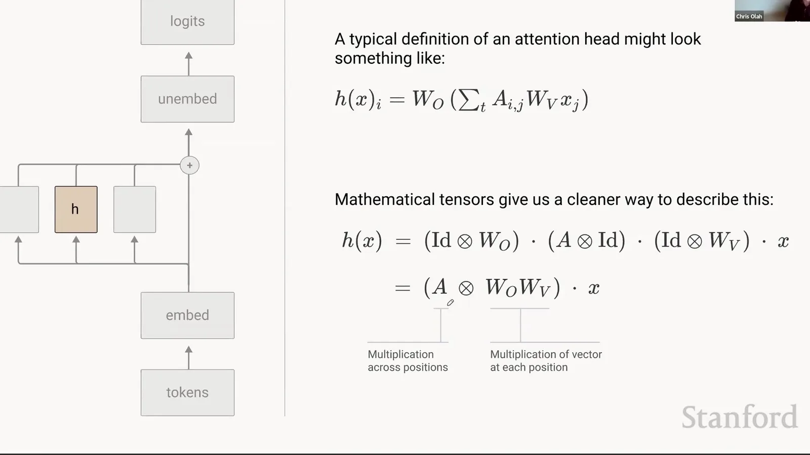
\teachervoice{讲者认为传统 \(Q,K,V,O\) 写法容易遮住 head 的结构。更有用的拆法是：\(A\) 负责决定信息从哪里移动到哪里，\(W_{OV}\) 负责决定究竟移动什么内容。}

Attention head 作为两个独立轴的算子

把 sequence-position mixing 与 feature-channel mapping 分开，可以把 head 看作 tensor/Kronecker product：

\[ h(X)=A^h(X)XW_{OV}^h \quad\Longleftrightarrow\quad \mathcal{H}^h=A^h\otimes W_{OV}^h. \]

左乘 \(A^h\)：在 positions 之间做 weighted sum；
右乘 \(W_{OV}^h\)：在 residual feature space 中读写；
两者的参数与语义可分别检查；
但 \(A^h\) 本身依赖输入，因此完整 head 仍非线性。

\lecturefigure{slide-13-attention-head-tensor-product.jpg}{单个 attention head：position mixing \(A^h\) 与 content map \(W_{OV}^h\)。}{Stanford Online 官方视频 00:18:14--00:18:31。}

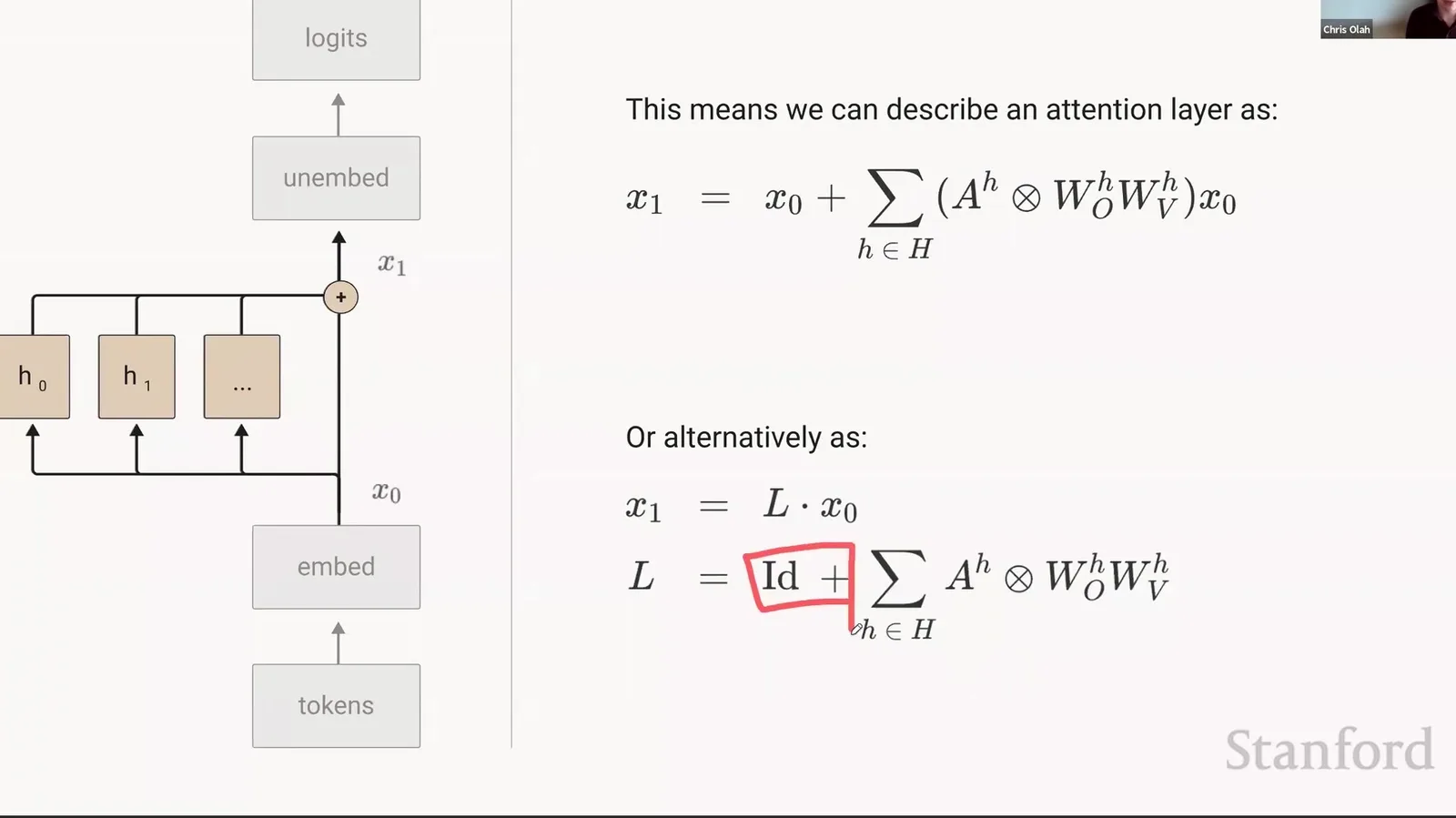
\lecturefigure{slide-14-attention-layer-sum.jpg}{一层 attention：identity residual path 加上全部 head operators。}{Stanford Online 官方视频 00:18:32--00:19:25。}

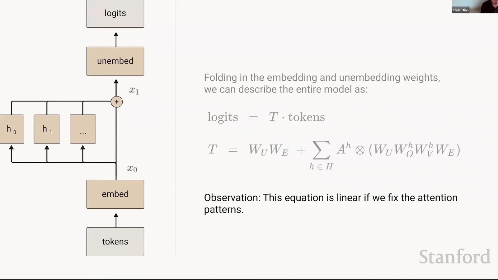
这张图中 \(I\) 不是普通装饰，而是 residual path。它让 token 的原始表示可以直接到达 unembedding，也让后续多层展开自然形成“选择某一层 head 或绕过它”的 path combinatorics。

Fold embedding 与 unembedding

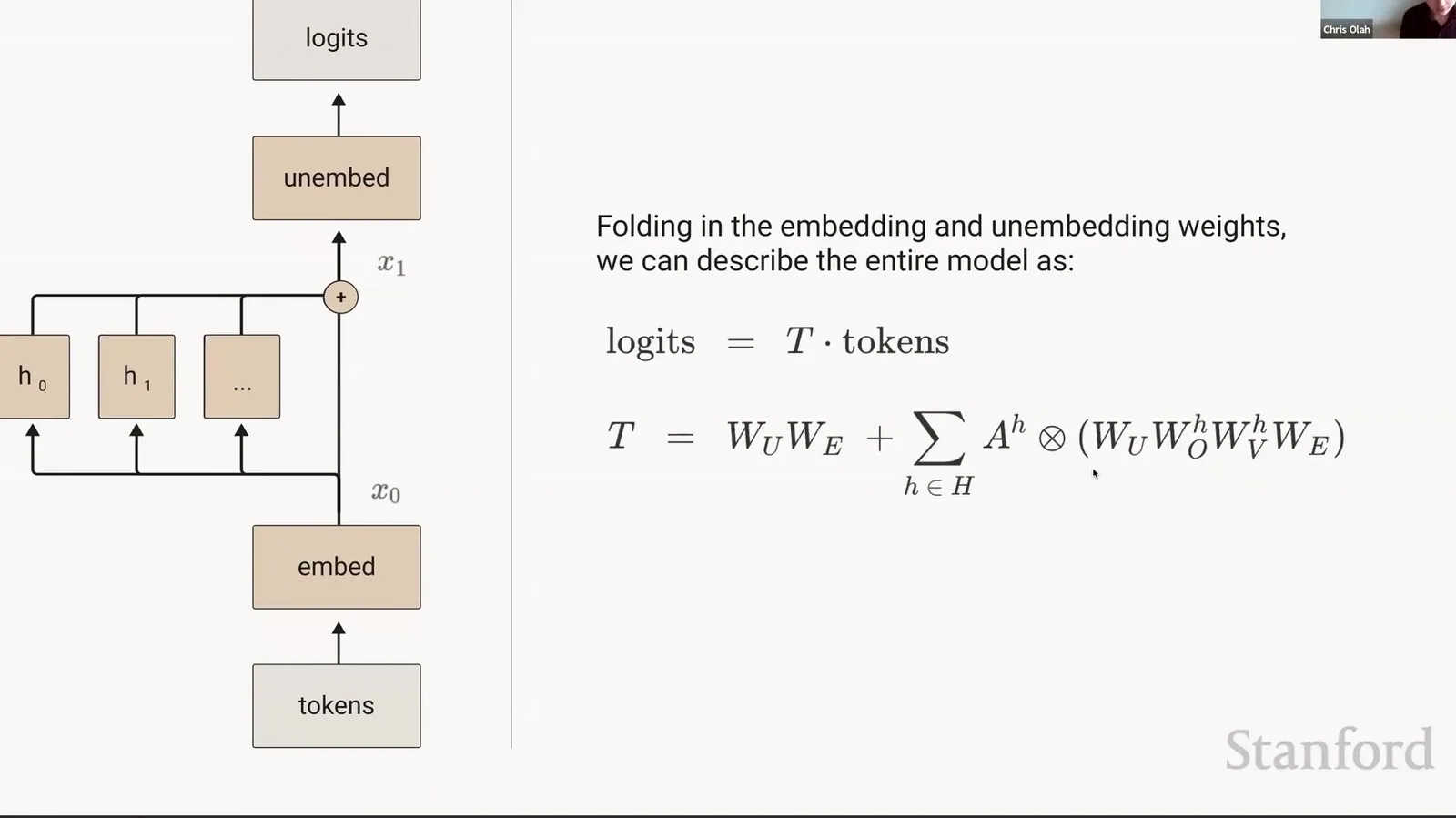
前面已经把一个 head 拆成 position routing 与 feature mapping，但读者最终关心的是 output-token logits，而不是抽象 residual coordinates。本节因此把输入端 embedding 和输出端 unembedding 折叠进各条路径，直接追问：某个 source token 被读取后，会提高或压低哪些候选 next tokens？这种 token-to-token 表示也为后面的 QK/OV circuit 检查建立统一接口。

把 \(W_E\)、\(W_U\) 与每个 head 合并，可以直接得到 vocabulary-to-vocabulary map：

\[ \mathrm{logits} =T W_EW_U +\sum_h A^h(T) T\underbrace{W_EW_{OV}^hW_U}_{M_{OV}^h}. \]

\(W_EW_U\)：direct path，主要存储 bigram-like statistics；
\(M_{OV}^h\in\mathbb{R}^{|V|\times |V|}\)：看到某 source token 后，该 head 对 output-token logits 的影响；
\(A^h\) 决定从哪个 source position 读取；
one-layer model 的可解释单元因此变成“attention pattern × token-to-token map”。

\lecturefigure{slide-15-fold-embedding-unembedding.jpg}{将 embedding/unembedding 折叠后，模型分为 direct/bigram path 与 head paths。}{Stanford Online 官方视频 00:19:26--00:19:35。}

\lecturefigure{slide-16-fixed-pattern-linearity.jpg}{关键观察：若固定 attention patterns，one-layer attention-only model 对输入是线性的。}{Stanford Online 官方视频 00:19:36--00:20:07。}

“固定 pattern 后线性”意味着什么

完整模型仍通过 softmax attention 依赖输入而非线性；但对某个具体 prompt 或一小类稳定 pattern，我们可以暂时把 \(A^h\) 当常量，再用线性代数分析 content path。Mechanistic analysis 常利用这种局部条件化，而不是声称 Transformer 全局线性。

\teachervoice{Olah 的方法论是：只要能把某一部分固定并转成线性，就获得了强大的解释工具。关键是诚实记录“固定了什么”，不能把 conditional linearity 偷换成 global linearity。}

本章小结

一层 attention-only Transformer 可以展开成 residual direct path 与每个 head 的加法项。Tensor-product 视角把“哪里读写”与“读写什么”分开；折叠 embedding/unembedding 后，每个 head 对 vocabulary logits 的作用可以直接检查。

QK 与 OV Circuits：一层模型究竟学了什么规则

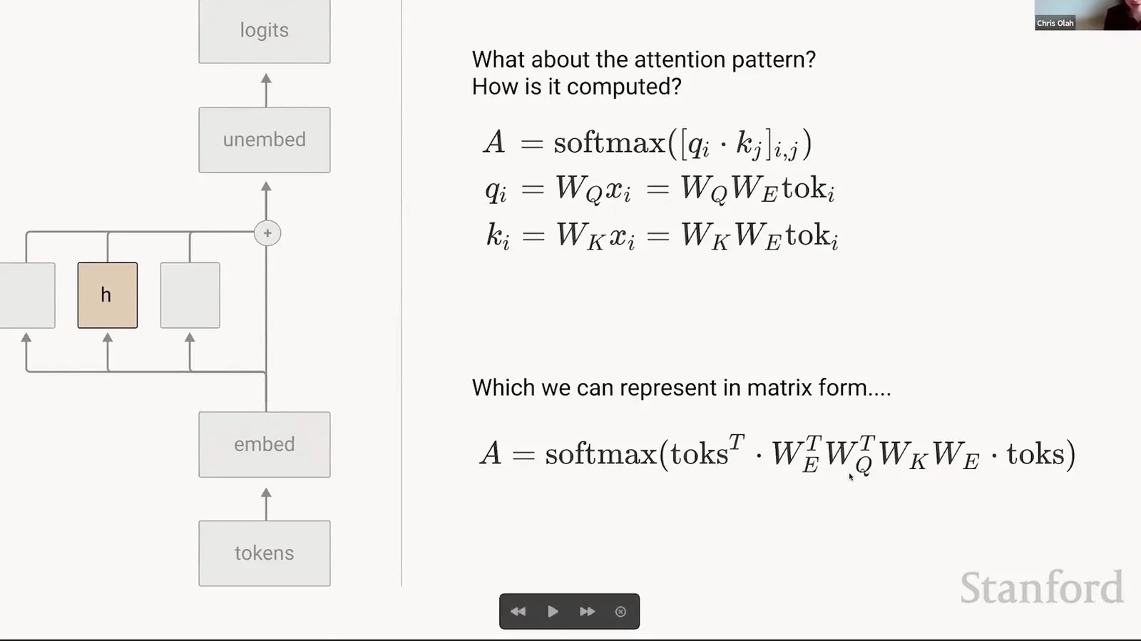
上一节只把 \(A^h\) 当作给定矩阵，现在需要解释 pattern 如何产生。对 row-vector convention，定义

\[ W_{QK}^h=W_Q^h(W_K^h)^{\top}, \qquad A^h=\operatorname{softmax}\!\left(XW_{QK}^hX^{\top}+M_{\mathrm{causal}}\right). \]

\(W_{QK}^h\)：决定 destination/query 与 source/key 的 compatibility；
\(W_{OV}^h\)：决定 source residual 被映射成什么写入；
\(M_{\mathrm{causal}}\)：屏蔽未来 positions；
一个 head 的功能必须同时描述 routing 与 writing。

\lecturefigure{slide-17-attention-pattern-qk.jpg}{Attention pattern 的计算：QK circuit 将 token/residual pairs 映射为 routing scores。}{Stanford Online 官方视频 00:20:08--00:20:39。}

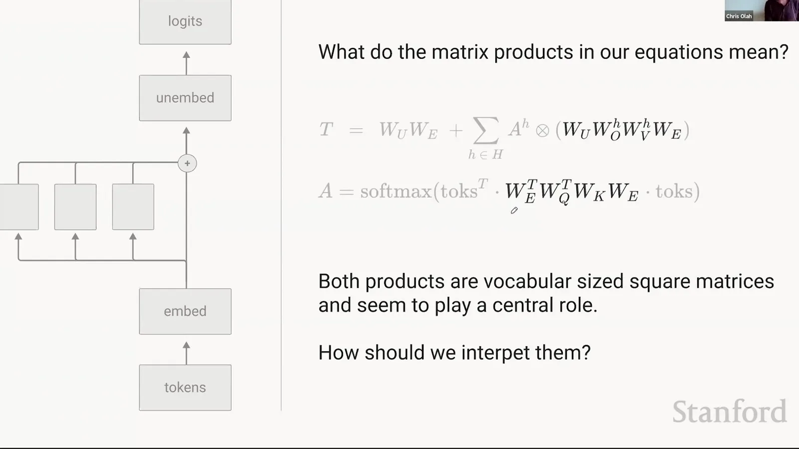
把 QK/OV 都投影到 vocabulary space

若忽略 contextual residual contribution，可定义有效 token-space matrices：

\[ M_{QK}^h=W_EW_{QK}^hW_E^{\top}, \qquad M_{OV}^h=W_EW_{OV}^hW_U. \]

\(M_{QK}^h[a,b]\)：destination token \(a\) 对 source token \(b\) 的相对偏好；
\(M_{OV}^h[b,c]\)：读取 source token \(b\) 后对 output token \(c\) 的 logit effect；
两个矩阵都是 vocabulary-sized，通常巨大；
positional embedding 与 prior-layer residual 会让实际 score 超出纯 token lookup。

\lecturefigure{slide-18-vocabulary-square-matrices.jpg}{QK 与 OV 折叠后都是 vocabulary-sized square matrices。}{Stanford Online 官方视频 00:20:40--00:24:29。}

\lecturefigure{slide-19-qk-ov-circuits.jpg}{Head 的两半：QK 连接 source/destination，OV 连接 attended token/output token。}{Stanford Online 官方视频 00:24:30--00:24:45。}

读图：不要把四种 token 角色混成两个

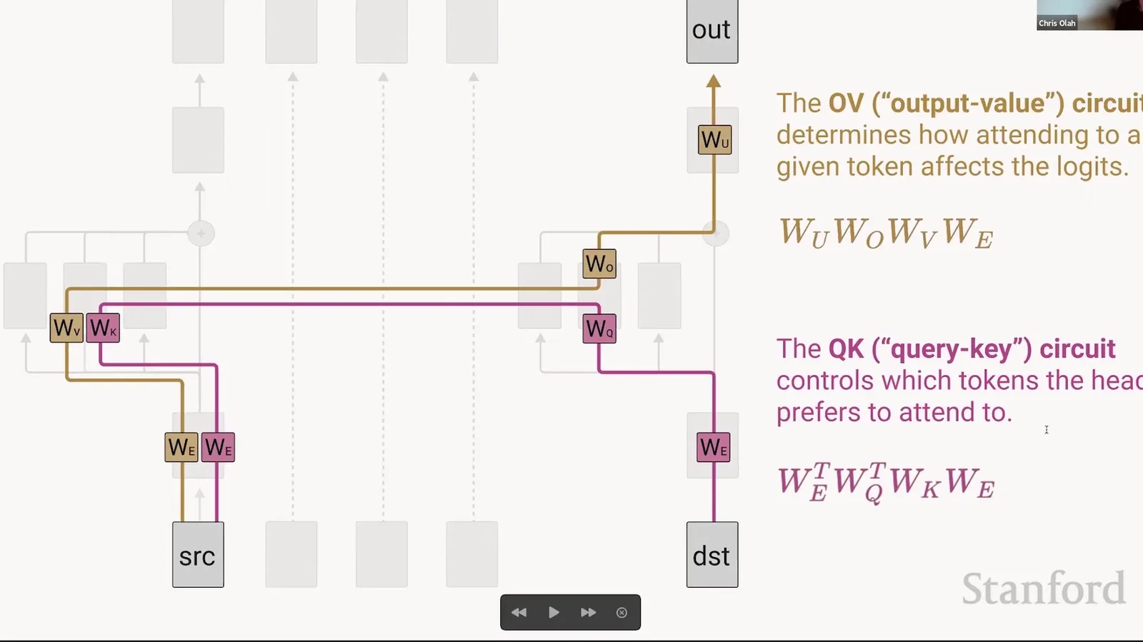
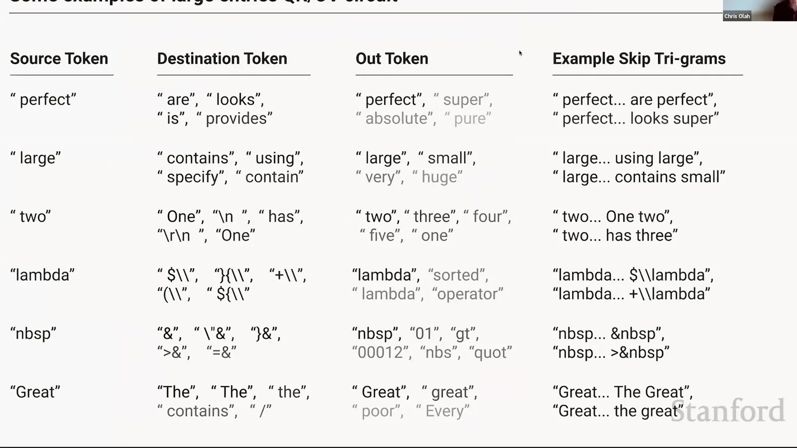
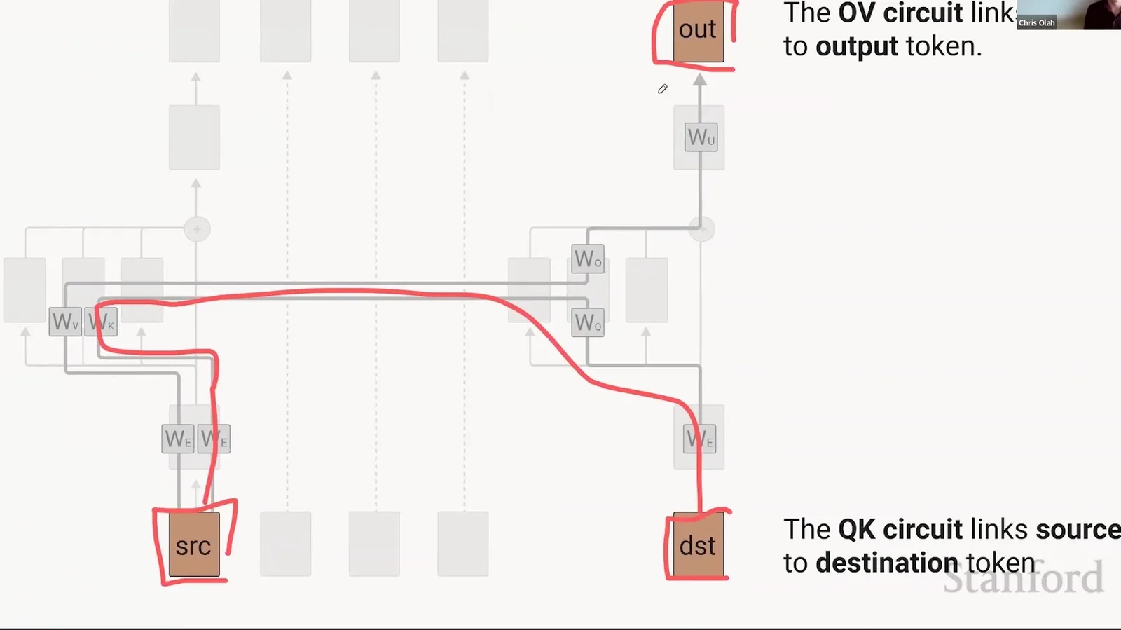
Source token 是被读取位置的内容；destination token 是当前更新的位置；out token 是 head 写入后被提升或压低的预测 token；最终 next token 还要经过其他 paths 共同决定。QK 主要连接前两者，OV 主要连接 source 与 out。

\teachervoice{讲者的直觉是 OV 更直接接受 output loss supervision：它决定写入哪些 logits；QK 通过“应该去哪里取信息”被间接训练。这个区分帮助读 dense matrix，但不意味着 QK 完全 unsupervised。}

Skip Trigram：一层 head 的基本规则

One-layer attention head 只能依据当前 destination representation 与候选 source representation 选择位置，然后用 source token 决定 output。它因此自然形成 skip-trigram rule：

\[ (\text{source token},\ \text{destination token}) \longrightarrow \text{out token}. \]

例如 destination 看到 “looks”，QK 可能偏向 earlier “perfect”，OV 再提升 “perfect” 或与之相关的 completion。

\lecturefigure{slide-20-skip-trigram-examples.jpg}{QK/OV 组合形成 example skip trigrams。}{Stanford Online 官方视频 00:24:46--00:25:05。}

\lecturefigure{slide-21-qk-source-destination.jpg}{QK circuit 明确链接 source token 与 destination token。}{Stanford Online 官方视频 00:25:06--00:27:47。}

为什么叫 skip trigram

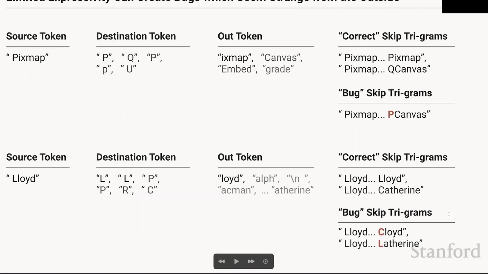
普通 trigram 依赖连续两个过去 tokens；这里 source 与 destination 可以相隔很远，中间被“skip”。规则仍只使用两个 token identities 决定第三个 output，因此表达力有限。

有限表达力会产生外部看来很奇怪的 bug

模型希望利用长距离 context，却只有 source/destination token pair 这个接口。它可能学到统计上常有用、但缺乏更丰富条件的规则，例如看到 rare technical token 后在若干可能位置盲目提升重复 token；当同一个 pair 在不同语境应产生不同 completion 时，one-layer head 无法区分。

\lecturefigure{slide-22-correct-skip-trigrams.jpg}{模型学到的“正确”skip trigrams 与受限规则。}{Stanford Online 官方视频 00:27:48--00:32:33。}

\lecturefigure{slide-23-qk-ov-composition-patterns.jpg}{一层模型可表达的 pattern family：source/destination matching 与 output mapping。}{Stanford Online 官方视频 00:32:34--00:32:57。}

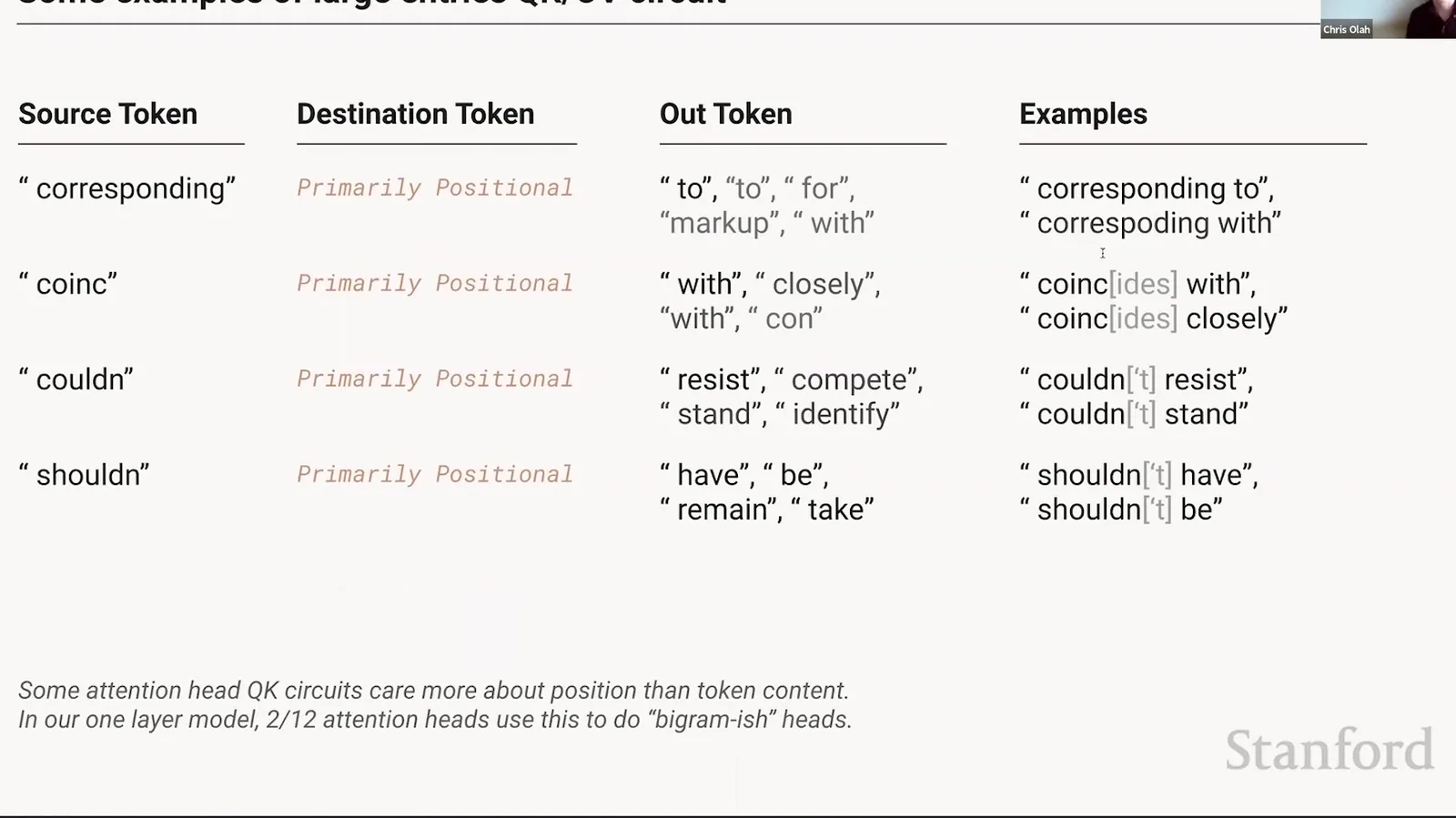
\lecturefigure{slide-24-positional-circuits.jpg}{部分 heads 主要编码 positional relations，而非纯语义 token pairs。}{Stanford Online 官方视频 00:32:58--00:33:31。}

读图：Primarily Positional 不等于“无意义”

Local/previous-token/offset heads 可以为后续 heads 移动位置标签、短语状态或邻接信息。单独看它们对 logits 的 marginal effect 可能不大，但在多层 composition 中可能成为关键 upstream component。

One-layer model 的行为边界

一层 attention-only models 确实会获得少量 ICL，课堂给出的量级约为 \(0.1\) nats，而不是两层模型约 \(0.4\) nats；它们也不经历前述 sharp phase change。这个差异提示：单 head 的 skip-trigram rules 不足以实现更强 pattern completion，需要多层 composition。

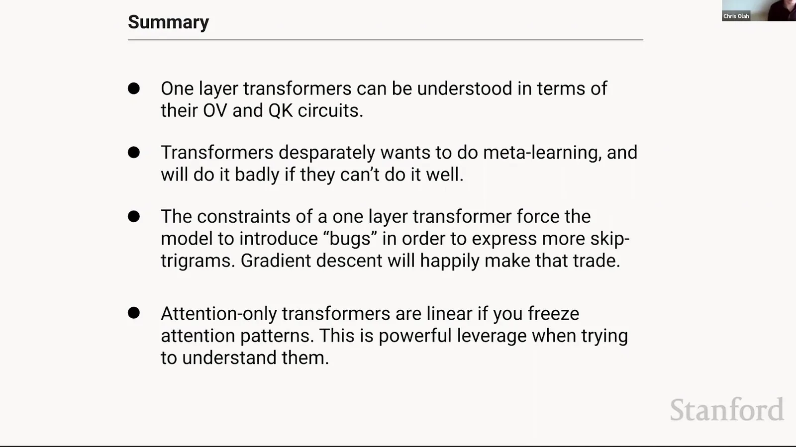
\lecturefigure{slide-25-one-layer-summary.jpg}{One-layer summary：QK/OV 可解释、skip trigrams 有用但受限、固定 pattern 后线性。}{Stanford Online 官方视频 00:33:32--00:33:57。}

\teachervoice{Olah 说 Transformers “desperately want” to use long context，因为远处信息能减少大量 entropy；一层模型被架构限制，只能用容易出 bug 的粗糙规则去追求这个目标。}

本章小结

QK circuit 决定 source/destination routing，OV circuit 决定 attended token 对 output logits 的写入。一层模型因此可被读成 skip-trigram 与 positional rules；这些 rules 能利用长 context，却缺少根据前文动态构造 richer match 的能力。

Eigenvalue Lens：从巨大 vocabulary matrix 压缩出 copying signature

上一章已经把 head 折叠成 token-to-token matrices，但这只是把问题变得可定义，还没有让它变得可阅读：\(M_{OV}\) 与 \(M_{QK}\) 的边长等于 vocabulary size，逐项枚举既昂贵，也很难形成全局判断。本节引入 eigenvalue lens，核心问题是能否用少量 spectral signatures 判断一个 head 更像 copying、anti-copying，还是 different-token mapping；读图时还要始终记住，这种压缩会丢失具体 token、basis 与非线性上下文。

若矩阵把同一向量空间映射回自身，可以用 eigenvectors/eigenvalues 总结它在某些 directions 上是放大、反转还是旋转。

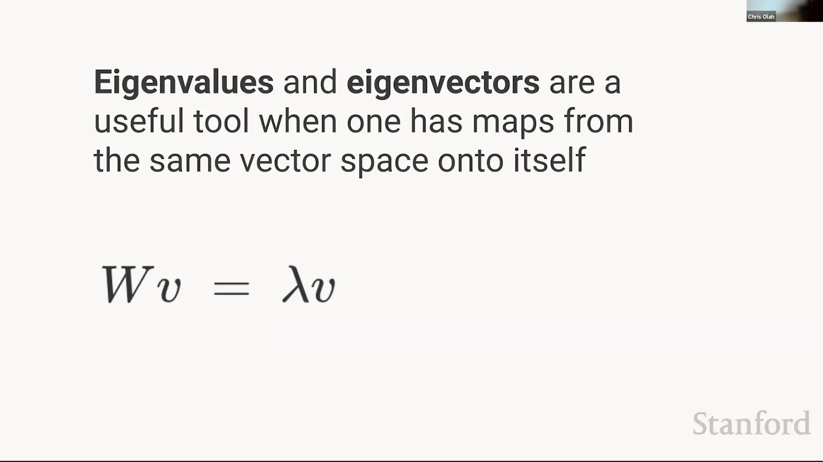
\lecturefigure{slide-26-eigenvector-introduction.jpg}{当输入输出属于同一空间时，eigenvectors 可压缩矩阵行为。}{Stanford Online 官方视频 00:33:58--00:34:21。}

\[ Mv=\lambda v. \]

\(v\)：矩阵作用后方向保持不变的 mode；
\(\lambda\)：该 mode 的缩放/相位变化；
real positive \(\lambda\)：沿同一方向增强；
real negative \(\lambda\)：反向抑制；complex \(\lambda\)：在二维子空间旋转并缩放。

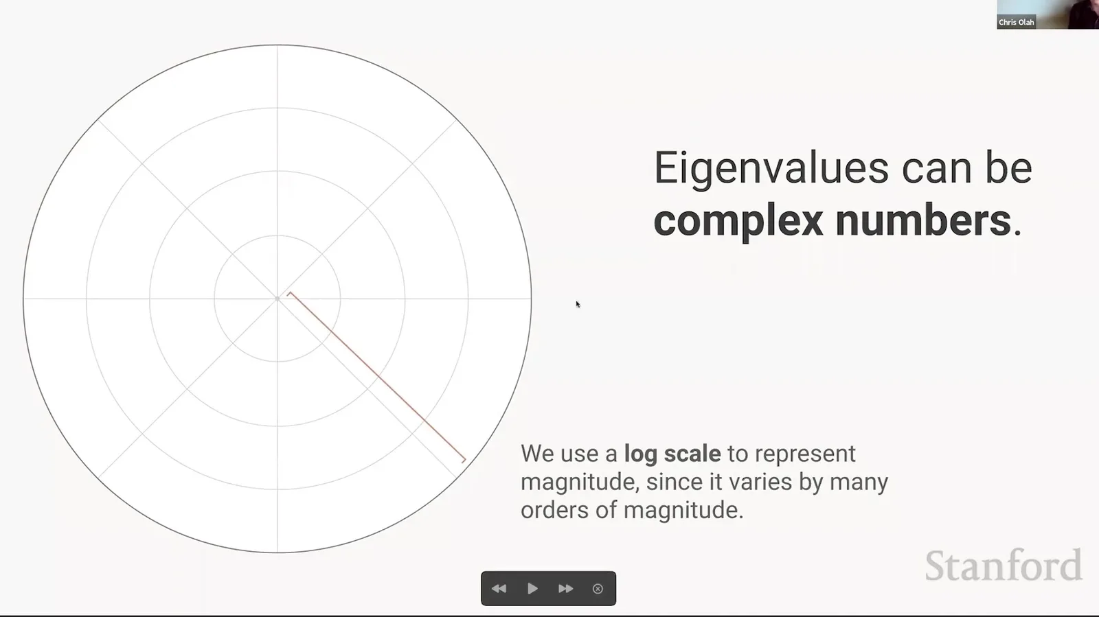
\lecturefigure{slide-27-complex-eigenvalues.jpg}{非对称 token-to-token maps 可以拥有 complex eigenvalues。}{Stanford Online 官方视频 00:34:22--00:35:09。}

OV spectrum 与 copying

对 token-space OV map，正 eigenmodes 表示看到某组 token directions 后提高同类 output directions 的 logits，可解释为 copying tendency；负 modes 是 anti-copying；complex/imaginary modes 更偏向把一种 token direction 映射到另一种。

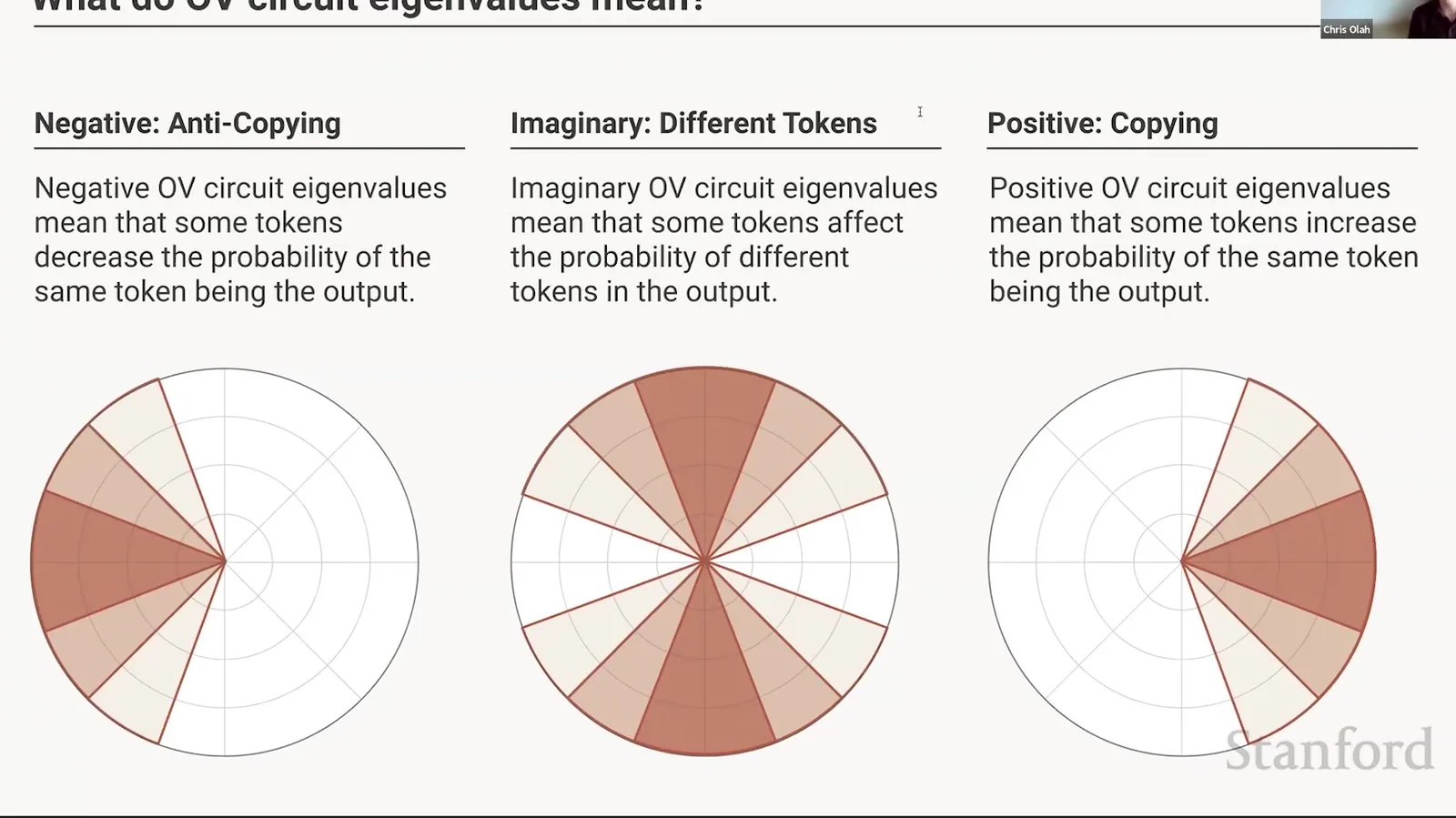
\lecturefigure{slide-28-ov-eigenvalue-meaning.jpg}{OV eigenvalue 图的教学解释：anti-copying、different-token mapping 与 copying。}{Stanford Online 官方视频 00:35:10--00:35:55。}

Spectrum 是 summary，不是完整语义字典

Vocabulary embedding/unembedding 不一定正交，矩阵也可能 non-normal；eigenvectors 未必对应单个可命名 token。将正 eigenvalue 简化为 copying 是对 small attention-only circuits 的实用诊断，不是对任意矩阵的普遍语义定理。

一层与两层 heads 的 copying distribution

Olah 展示一层模型中十个（共十二个）heads 的 OV spectrum 主要落在正实方向，说明模型大量使用“看到 token 后提升相同/相关 token”这一简单策略。两层模型中也有大量 copying heads，但多层 routing 允许它们被更精确的 pattern 触发。

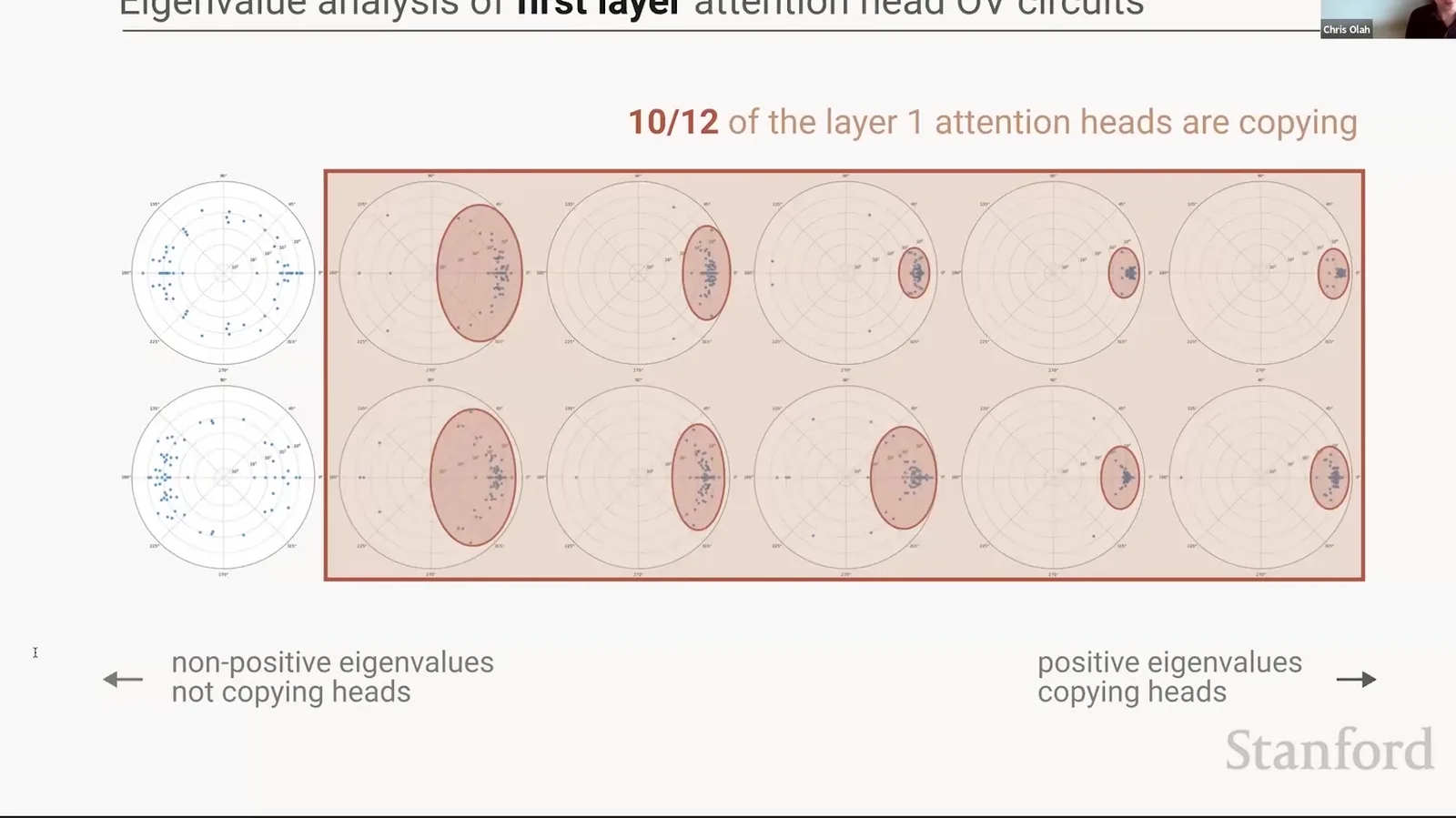
\lecturefigure{slide-29-layer-one-copying-heads.jpg}{一层模型：10/12 attention heads 具有强 copying signature。}{Stanford Online 官方视频 00:35:56--00:36:05。}

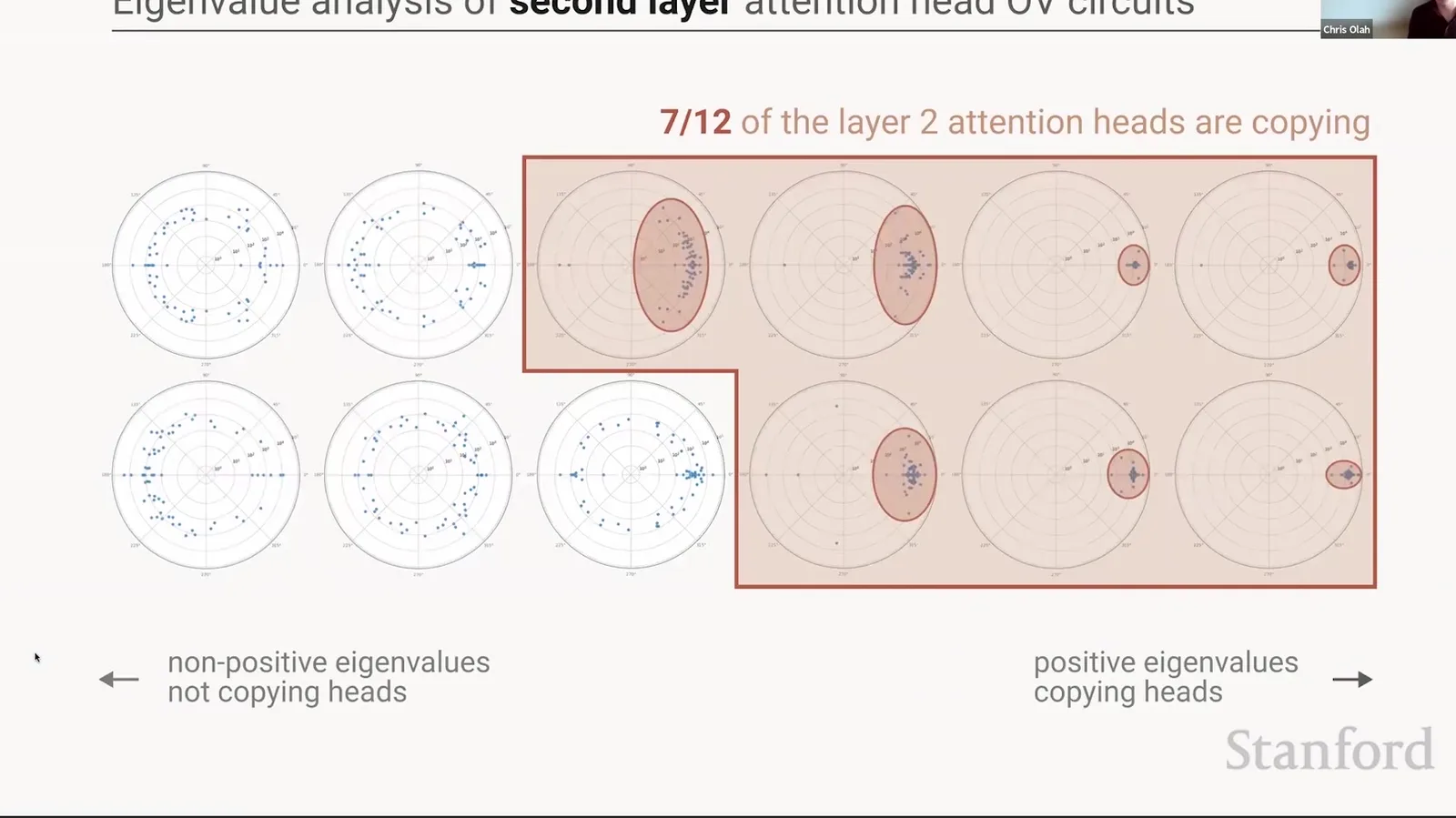
\lecturefigure{slide-30-layer-two-copying-heads.jpg}{两层模型：第二层仍有多个强 copying heads。}{Stanford Online 官方视频 00:36:06--00:36:41。}

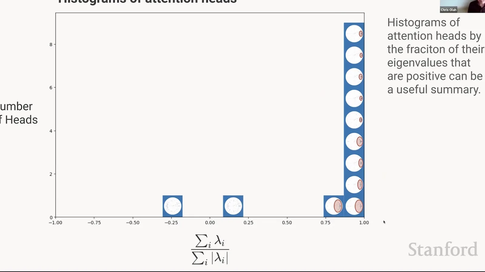
\lecturefigure{slide-31-head-eigenvalue-histogram.jpg}{把 OV spectral signature 压缩为全模型 head histogram。}{Stanford Online 官方视频 00:36:42--00:37:21。}

\teachervoice{讲者强调这是 bottom-up methodology：先从矩阵结构推导可读 summary，再说“这些 heads 多数在 copy”，而不是先假设所有 heads 都是某类 pattern 后去挑支持例子。}

QK spectrum 与方法失效边界

QK 的 positive mode 倾向匹配相同 token direction，negative mode 倾向避免相同 token，complex mode 倾向不同-token relation。它在多层模型中更有意义，因为 previous heads 可以把“前一个 token 是什么”等信息写入当前 residual，再由下一层 QK 做 same-feature matching。

\lecturefigure{slide-32-qk-eigenvalues-multilayer.jpg}{QK eigenvalues 在多层 chains 中更有用：前层先移动信息，后层再匹配。}{Stanford Online 官方视频 00:37:22--00:37:37。}

\lecturefigure{slide-33-eigenanalysis-breaks-at-scale.jpg}{Naive eigenvalue analysis 随模型增大和加入 MLP 而失效。}{Stanford Online 官方视频 00:37:38--00:38:35。}

MLP 让“一个矩阵解释一切”失效

Attention-only model 在 fixed pattern 下可局部线性化；MLP 引入 activation-dependent nonlinear feature transforms，LayerNorm 也耦合坐标。大型模型仍可分析局部 Jacobian、features 与 paths，但不能直接把 small-model eigenvalue story 原样复制。

\teachervoice{Olah 明确说 naive spectral method 在加入 MLP 后 “completely breaks down”。高质量讲义必须保留这句话，不能把 eigenvalue plots 包装成通用 LLM interpretability toolkit。}

本章小结

Eigenvalue lens 将巨大 token-to-token circuit 压缩成 copying/anti-copying 等趋势，并揭示一层模型强烈依赖广泛 copying。它依赖同空间映射和近似线性结构，面对 MLP 与大模型时只能作为有限线索。

两层 Composition：从 Additive Heads 到 Virtual Heads

一层模型缺少 phase change，而两层模型拥有。区别不只在“多了一倍 heads”，更在于第二层 attention pattern 可以读取第一层写入的 features，并且两层 value paths 会组合成新的 effective operator。下面用 path expansion 把这种组合显式展开。

\lecturefigure{slide-34-one-layer-formula-recall.jpg}{回顾一层模型的 direct path 与 single-head paths。}{Stanford Online 官方视频 00:38:36--00:39:05。}

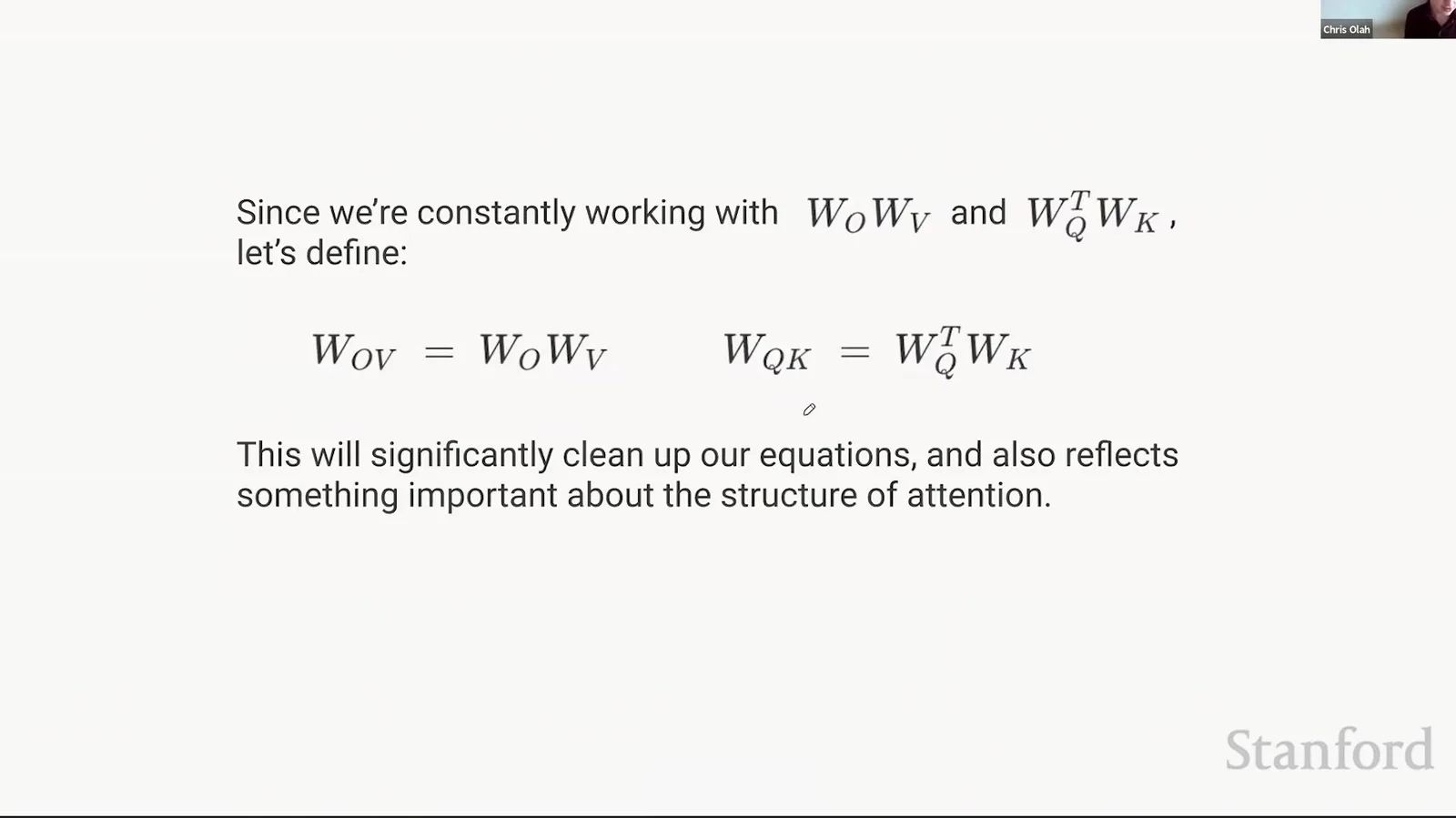
定义可复用的 OV 与 QK 矩阵

为了减少符号，文章与讲座把总是一起出现的 matrices 合并：

\[ W_{OV}^{\ell,h}=W_V^{\ell,h}W_O^{\ell,h}, \qquad W_{QK}^{\ell,h}=W_Q^{\ell,h}(W_K^{\ell,h})^{\top}. \]

其中 \(\ell\) 是 layer index，\(h\) 是 head index。前者描述 content write，后者描述 compatibility metric。

\lecturefigure{slide-35-define-wov-wqk.jpg}{定义 \(W_{OV}\) 与 \(W_{QK}\)，暴露 attention 的两类核心 circuit。}{Stanford Online 官方视频 00:39:06--00:39:33。}

两层模型的算子乘积

定义好单层的 \(W_{QK}\) 与 \(W_{OV}\) 后，接下来的问题不是简单地再写一遍第二层，而是解释第二层怎样使用第一层已经写入 residual stream 的信息。本节把两层视为两个 residual-plus-head operators 的乘积；这样既能保留每层的独立 heads，也能显式看见只有跨层组合才存在的 effective paths。这个展开是从“模型有两层”走向“模型获得新算法能力”的关键桥梁。

忽略 LayerNorm/MLP/bias，令每层 operator 为

\[ \mathcal{L}_{\ell} =I+\sum_{h\in H_{\ell}}A^{\ell,h}\otimes W_{OV}^{\ell,h}. \]

两层 residual transform 为

\[ X_2=\mathcal{L}_2\mathcal{L}_1X_0. \]

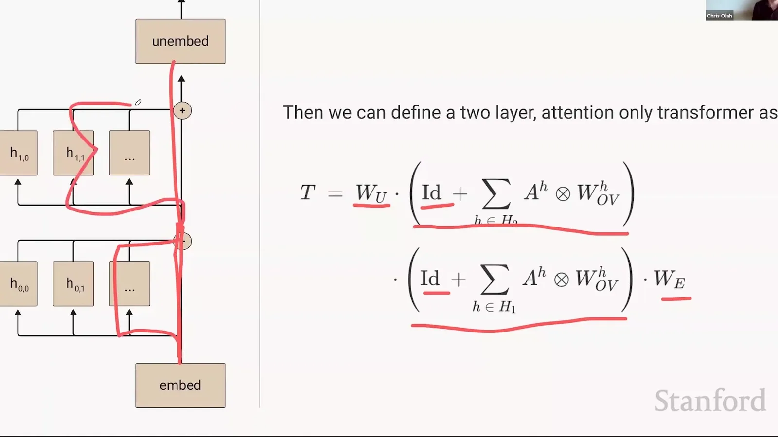
\lecturefigure{slide-36-two-layer-formula.jpg}{两层 attention-only Transformer：两个 residual-plus-head operators 相乘。}{Stanford Online 官方视频 00:39:34--00:39:59。}

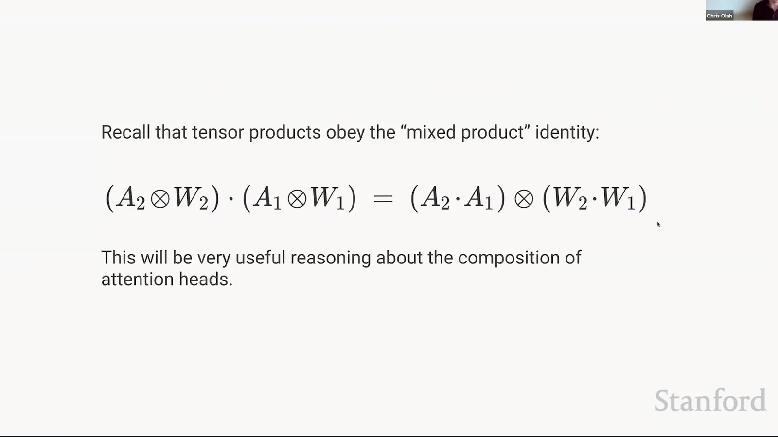
Kronecker product 满足 mixed-product identity：

\[ (A_2\otimes W_2)(A_1\otimes W_1) =(A_2A_1)\otimes(W_2W_1). \]

\(A_2A_1\)：position routing 的两步 composition；
\(W_2W_1\)：content transformation 的两步 composition；
identity 选择会产生绕过某层的 paths；
注意矩阵实际依赖 residual，因此符号展开不消除 routing nonlinearity。

\lecturefigure{slide-37-mixed-product-identity.jpg}{Mixed-product identity 将 position composition 与 content composition 分开。}{Stanford Online 官方视频 00:40:00--00:40:33。}

展开后的三类路径

算子乘积本身还没有告诉我们哪些计算路径真正出现。本节进一步展开 \(\mathcal{L}_2\mathcal{L}_1\)，并按是否绕过某层、只经过单个 head、或连续经过两层 heads 来分类。读下面的式子时，应把每一项看成一条可单独检查和干预的信息流，而不是把所有 summands 又压回一个黑箱矩阵；induction circuit 正是最后一类 composed path 的具体实例。

展开得到：

\[ I +\sum_{h\in H_1}A^{1,h}\otimes W_{OV}^{1,h} +\sum_{k\in H_2}A^{2,k}\otimes W_{OV}^{2,k} +\sum_{k,h}(A^{2,k}A^{1,h})\otimes (W_{OV}^{2,k}W_{OV}^{1,h}). \]

direct path：两层都走 residual；
single-head paths：只经过某一层的一个 head；
virtual/composed paths：第一层 head 的输出被第二层 head 读取；
virtual head 不是新增参数，而是已有 heads composition 的 effective circuit。

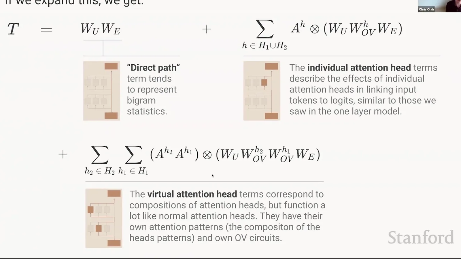
\lecturefigure{slide-38-expanded-two-layer-terms.jpg}{两层展开：direct、individual head 与 virtual-head composition terms。}{Stanford Online 官方视频 00:40:34--00:41:39。}

\lecturefigure{slide-39-principled-head-analysis.jpg}{Path expansion 提供原则化的 attention-head 分析框架。}{Stanford Online 官方视频 00:41:40--00:42:43。}

Circuit 不等于“单个 head”

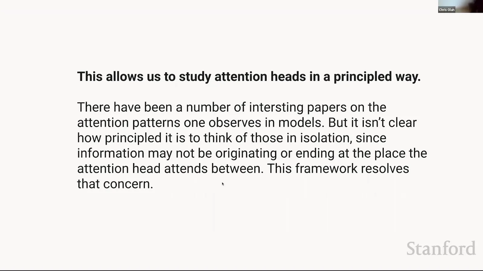
一个算法可以跨多个 heads 与 layers：上游 head 写入 feature，下游 head 用 QK 读取它，再由 OV 写入 logits。只按单-head attention map 命名容易漏掉 composition；path 是更接近程序执行的单位。

用 marginal loss accounting 排序 paths

Toy model 中可以 ablate 或移除 path term，测量对 loss 的边际影响。讲座给出 direct path、individual layer-one/two heads 与 virtual paths 的量级；许多虚拟项单独很小，但不应因此永久丢弃，因为它们可能在更深模型或特定 input 上成为关键。

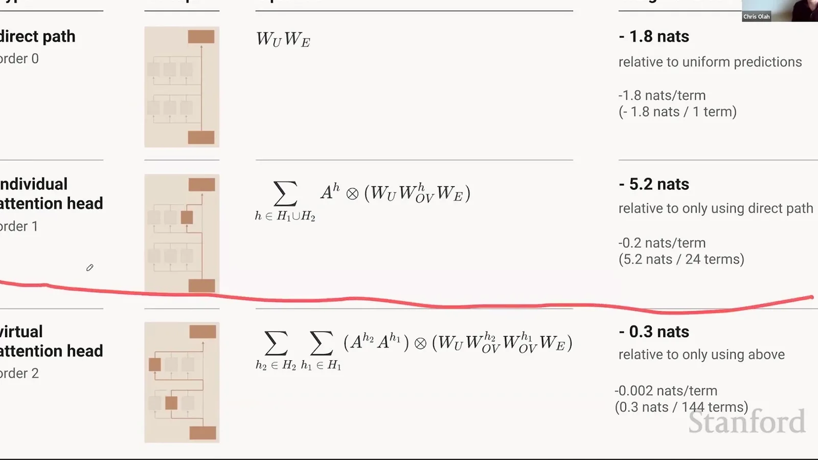
\lecturefigure{slide-40-path-loss-contributions.jpg}{不同 path types 对 loss 的 marginal contribution。}{Stanford Online 官方视频 00:42:44--00:42:49。}

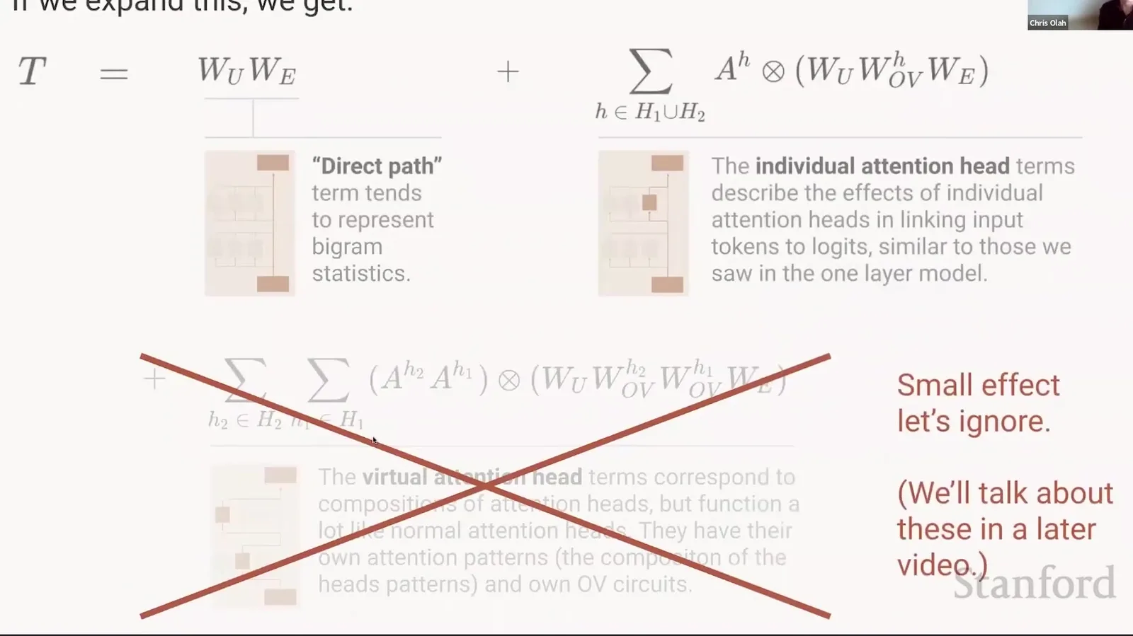
\lecturefigure{slide-41-virtual-heads-later.jpg}{当前模型中 virtual-head terms 较小，但在更深模型中可能重要。}{Stanford Online 官方视频 00:42:50--00:43:05。}

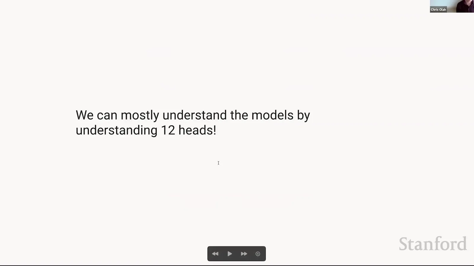
\lecturefigure{slide-42-understand-model-with-twelve-heads.jpg}{Near-complete toy-model accounting：主要行为可由约十二个 heads 理解。}{Stanford Online 官方视频 00:43:06--00:43:09。}

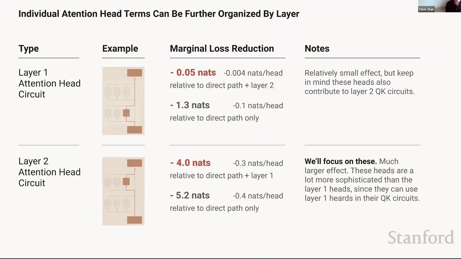
\lecturefigure{slide-43-head-terms-by-layer.jpg}{按 layer/type 组织 attention-head terms 与 loss reduction。}{Stanford Online 官方视频 00:43:10--00:43:21。}

读图：marginal effect 不是唯一重要性指标

Head ablation 可能被冗余路径补偿；一个上游 head 的 OV direct logit effect 很小，却可能强烈改变下游 QK routing。应同时看 direct logit effect、path composition、attention-pattern dependence 与 behavior-specific ablation。

第二层 pattern 依赖第一层写入

即使 OV path 可以形式化为加法，第二层的 \(Q\) 与 \(K\) 来自包含第一层 outputs 的 residual stream。因此第二层 attention pattern 本身包含 cross terms：previous heads 改变“去哪里看”，而不只改变“看完后写什么”。

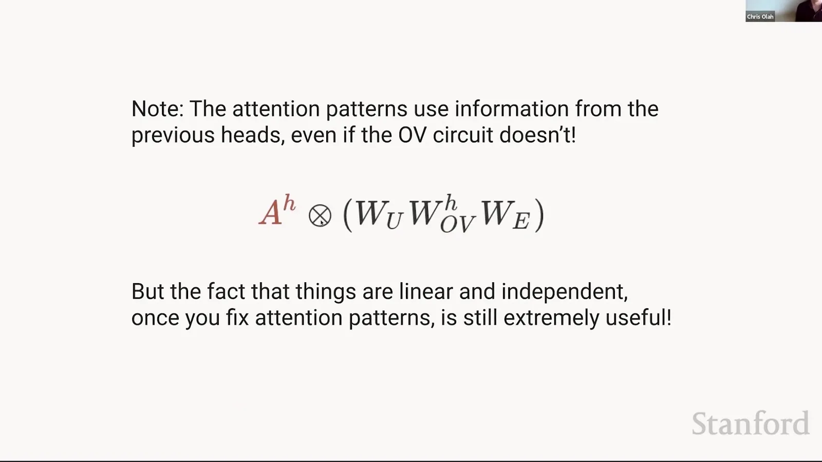
\lecturefigure{slide-44-patterns-read-previous-heads.jpg}{第二层 attention patterns 使用第一层信息，即使简单 OV path 暂时忽略 composition。}{Stanford Online 官方视频 00:43:22--00:43:39。}

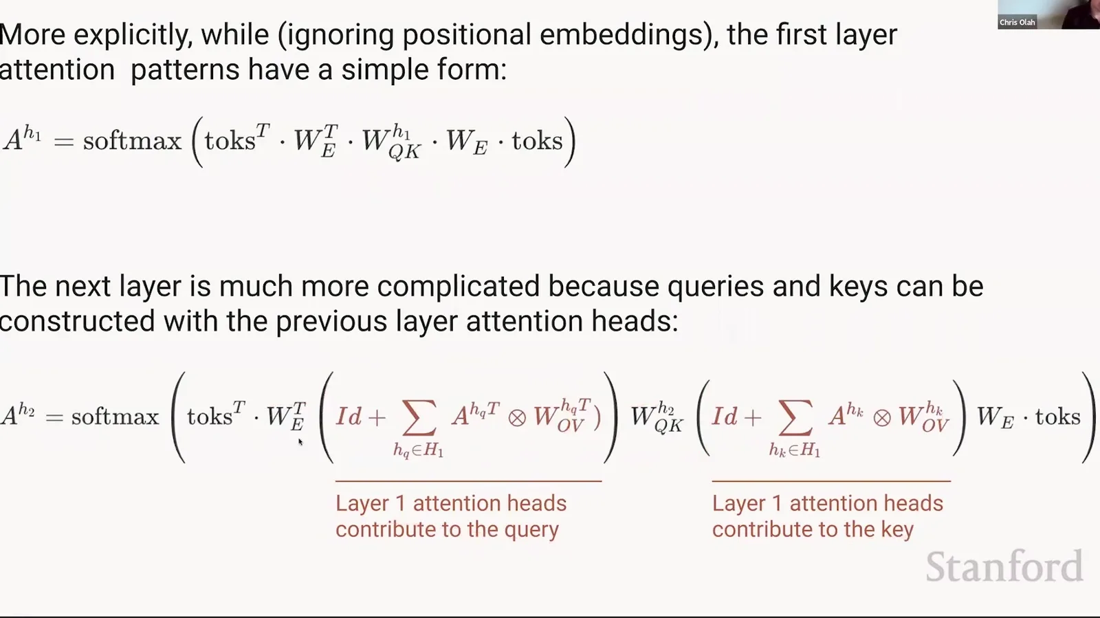
\lecturefigure{slide-45-layer-two-qk-context.jpg}{显式展开第二层 QK：queries/keys 都可包含第一层 heads 的贡献。}{Stanford Online 官方视频 00:43:40--00:43:49。}

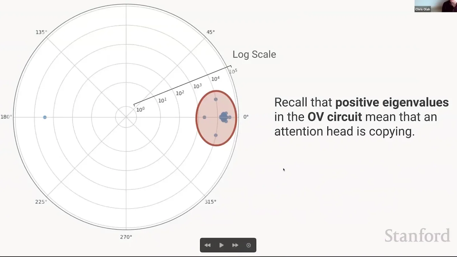
\lecturefigure{slide-46-positive-eigenvalues-copy.jpg}{复制型 OV signature：positive eigenvalues 使 attended token 更可能被输出。}{Stanford Online 官方视频 00:43:50--00:43:59。}

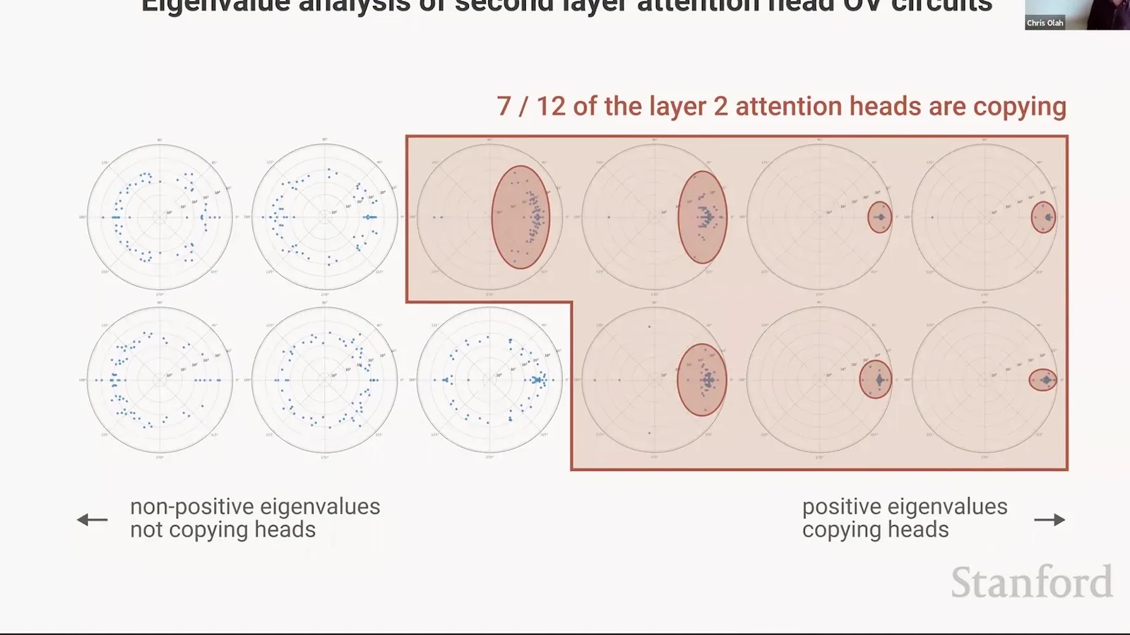
\lecturefigure{slide-47-second-layer-copying-circuits.jpg}{第二层多个 heads 具有 copying OV circuit，为 conditional copy 奠定基础。}{Stanford Online 官方视频 00:44:00--00:44:11。}

\lecturefigure{slide-48-inspect-patterns-empirically.jpg}{QK circuit 变复杂时，从 empirical attention patterns 反推候选机制。}{Stanford Online 官方视频 00:44:12--00:46:07。}

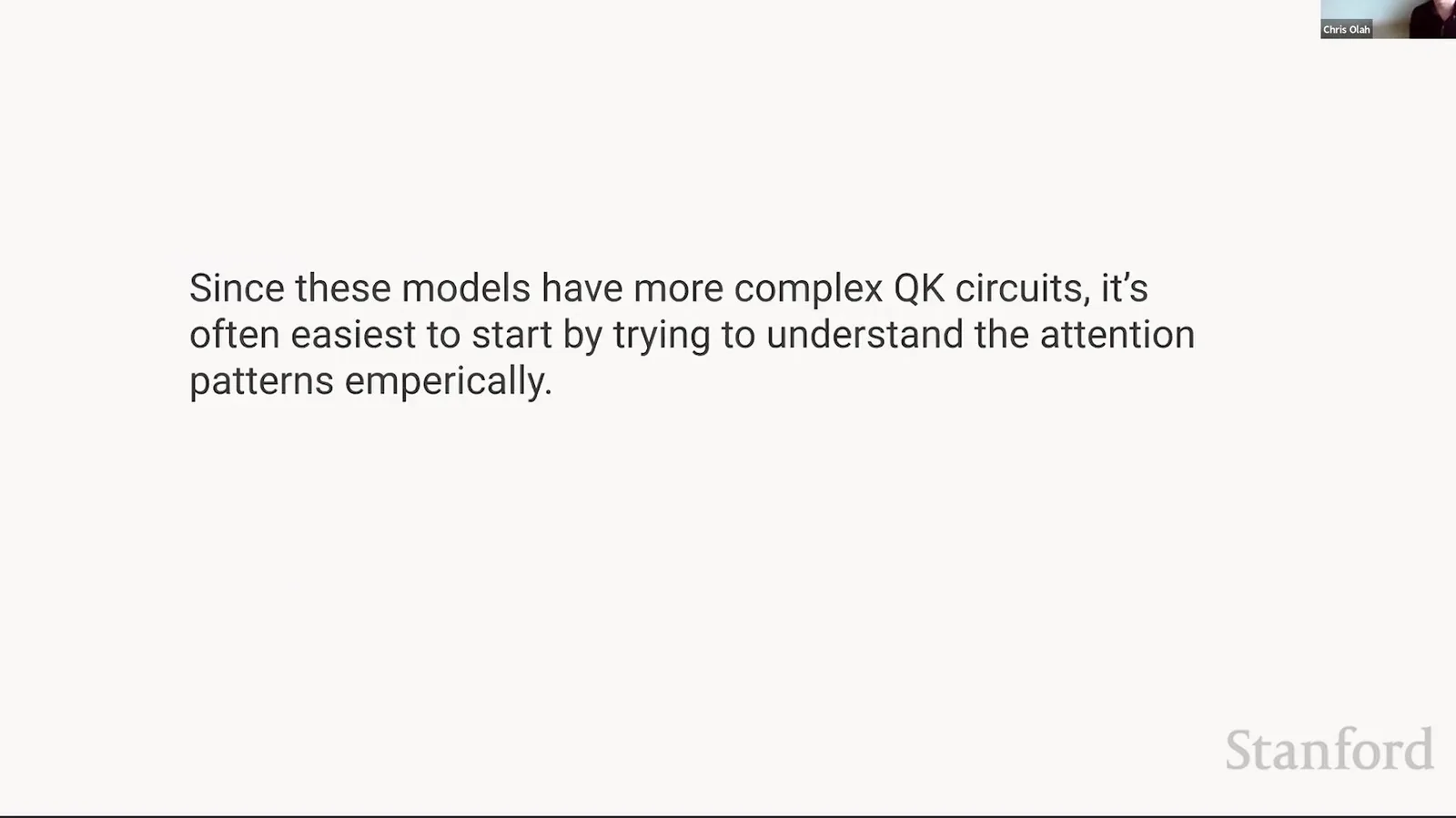
\teachervoice{Olah 既使用 algebra，也承认复杂 QK circuit 最容易从实际 attention pattern 开始看。Mechanistic interpretability 不是只准一种工具，而是让公式、visualization、ablation 与 examples 互相约束。}

本章小结

两层模型通过 operator multiplication 产生 direct、single-head 与 composed virtual paths。更重要的是，第一层写入会改变第二层 routing，使模型能先移动“前一个 token”等状态，再用下一层匹配并复制，从而获得一层模型不具备的 conditional algorithm。

Induction Heads：实现 In-Context Nearest Neighbor 的电路

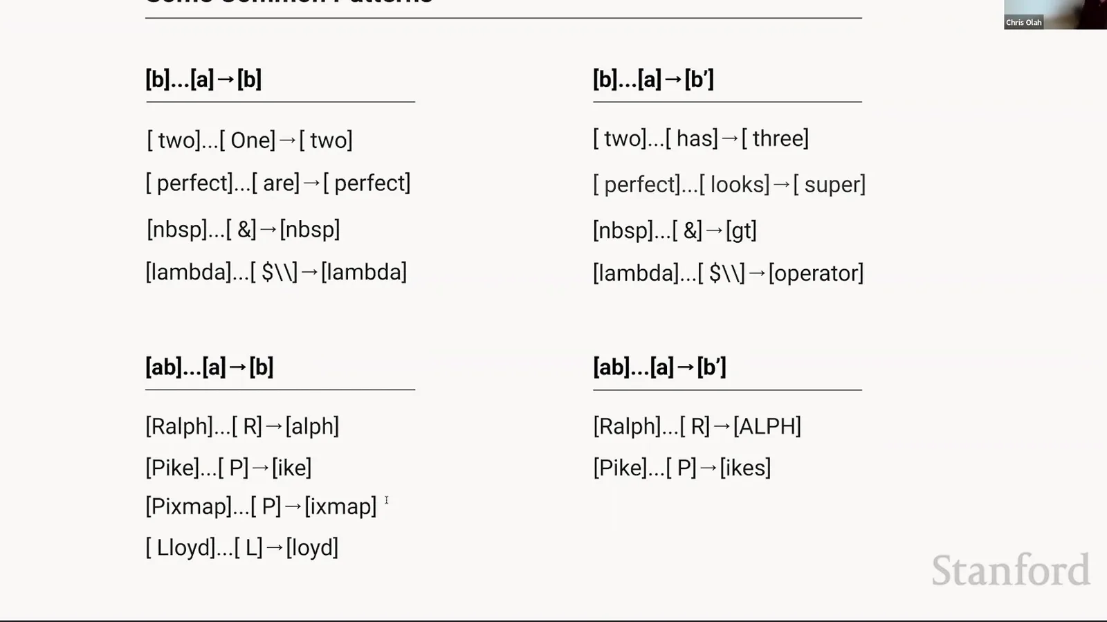
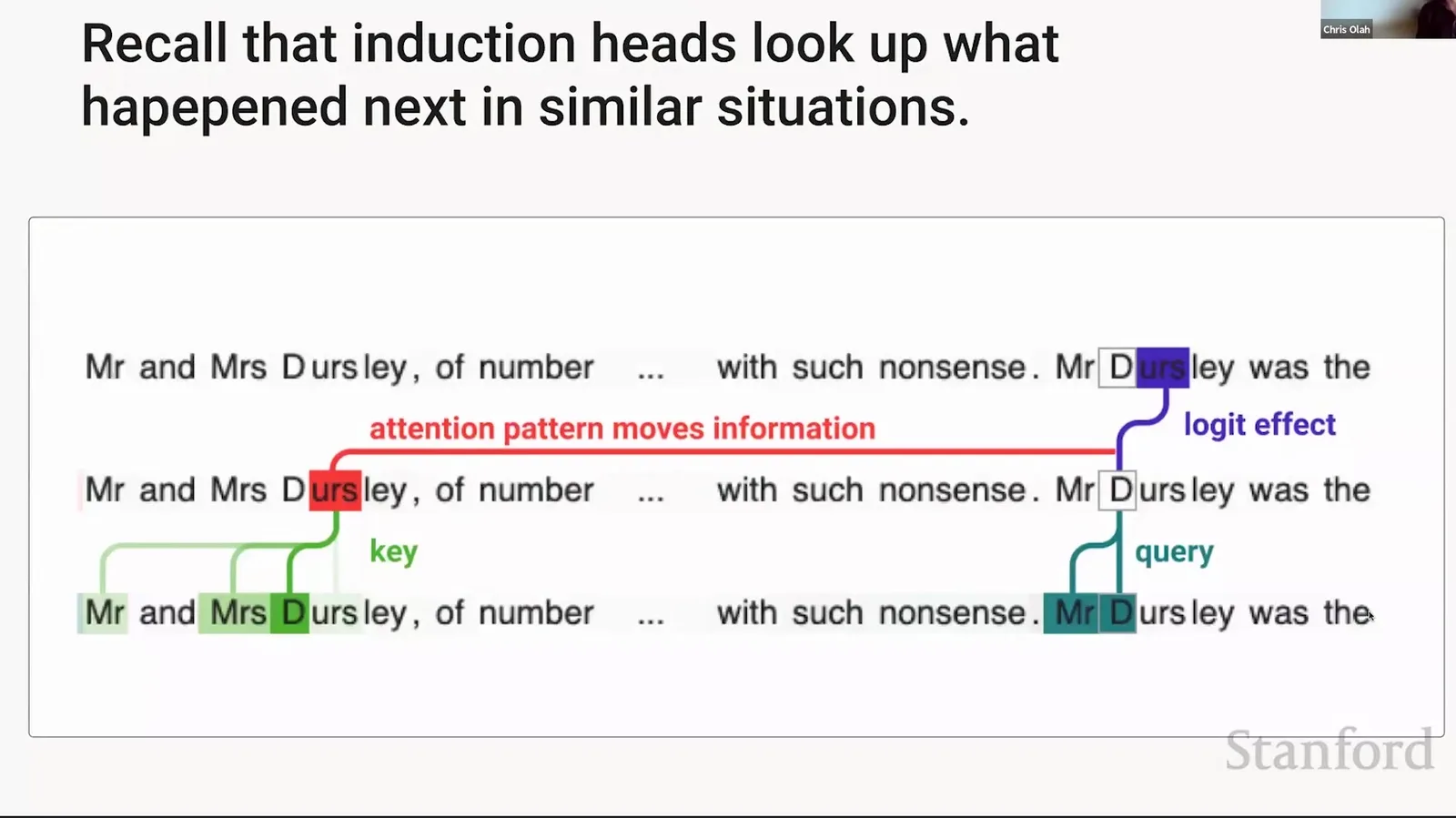
现在回到 phase-change mystery。一个 induction head 处理模式

\[ [A][B]\ \cdots\ [A]\quad\longrightarrow\quad[B]. \]

它在当前 token 为 \(A\) 时，寻找此前出现的 \(A\)，再读取那个旧 \(A\) 后面的 \(B\)，提升 \(B\) 的 next-token probability。

Induction pattern

机制通常需要两步 composition。Previous-token head 将位置 \(j-1\) 的 token identity 写入位置 \(j\)；下一层 induction head 在当前位置的 \(A\) 与候选位置所携带的 previous-token feature 之间做 QK match，并通过 copying OV 输出候选位置的当前 token \(B\)。

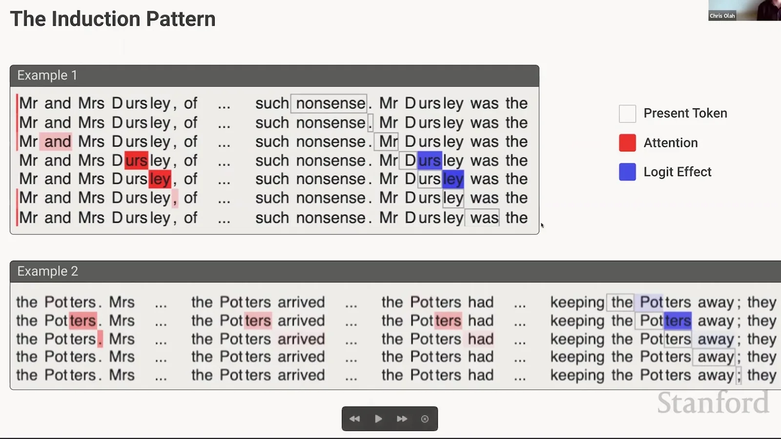
\lecturefigure{slide-49-induction-pattern.jpg}{Induction pattern：匹配此前相同 prefix，并复制它后面的 token。}{Stanford Online 官方视频 00:46:08--00:47:01。}

Induction-head algorithm 的概念性伪代码。

def induction_prediction(tokens, current_index):
    current_token = tokens[current_index]
    candidates = []
    for source in range(1, current_index):
        if tokens[source - 1] == current_token:
            candidates.append(tokens[source])
    return learned_weighted_copy(candidates)

In-context nearest neighbor

Induction head 把 context 当作临时数据库：query 是当前 pattern，keys 是历史 pattern，value 是历史 pattern 之后发生的 token。它与 k-NN 类似，但相似度、representation、组合路径与 output transformation 都由网络学习。

\teachervoice{Olah 的一句压缩定义是：寻找 previous copy，向前看一位，然后预测上次发生的事情会再次发生。实际 heads 可以匹配短语、token classes 或语义近邻，不只匹配字面完全相同的 \(A\)。}

为什么它是 meta-learning workhorse

简单 copying head 只会在很多可能位置盲目提升重复 token；induction circuit 则先识别“哪个过去情境与当前相似”，再复制该情境的 continuation。这个 conditional retrieval 更像一个可泛化的 context algorithm，因此能支持重复文本、格式模仿、局部函数学习与翻译对应。

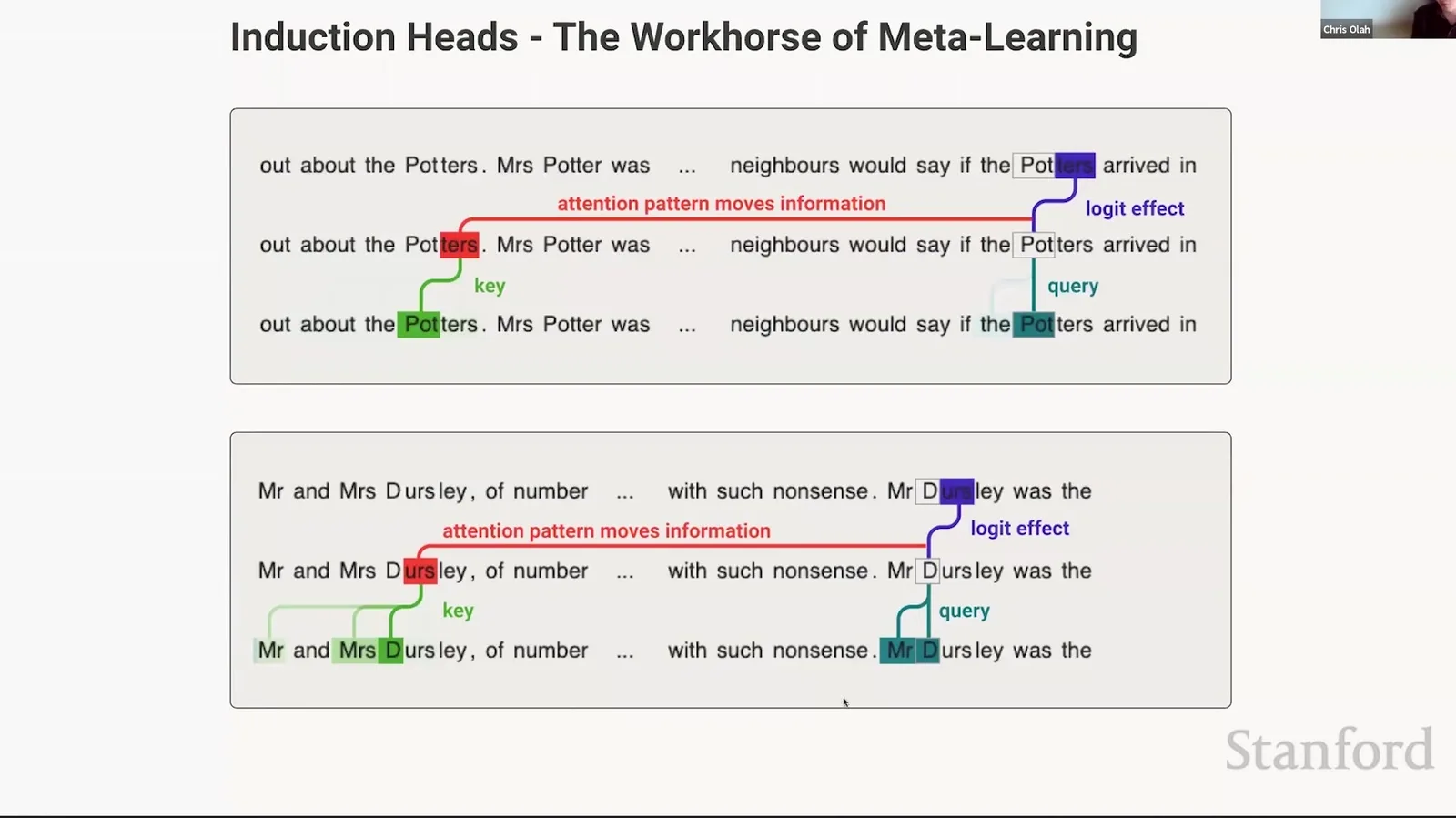
\lecturefigure{slide-50-induction-workhorse.jpg}{Induction heads：meta-learning 的 workhorse，组合 pattern matching 与 copying。}{Stanford Online 官方视频 00:47:02--00:47:05。}

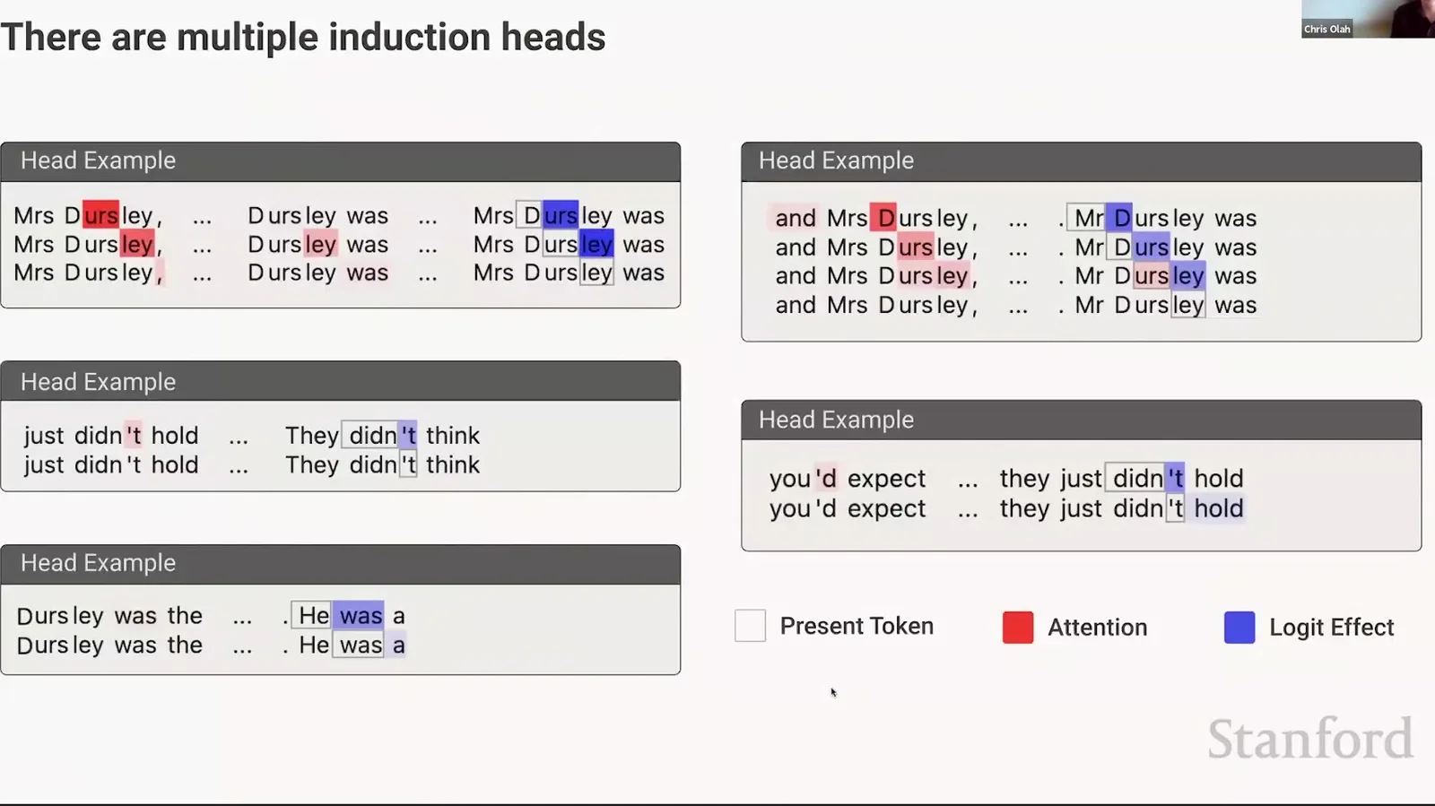
\lecturefigure{slide-51-multiple-induction-heads.jpg}{模型中存在多个 induction heads，覆盖不同 pattern 与 logit effects。}{Stanford Online 官方视频 00:47:06--00:47:29。}

从 attention pattern 到 matrix signature

对经典 induction head，OV 应具有 copying tendency；QK 应在 first-layer shifted feature 上偏好 same-token/same-pattern match。因此可以用 QK/OV traces 或 eigenvalue summaries把 heads 放入二维图：右上角同时具有 strong QK matching 与 OV copying 的 heads 是 induction candidates。

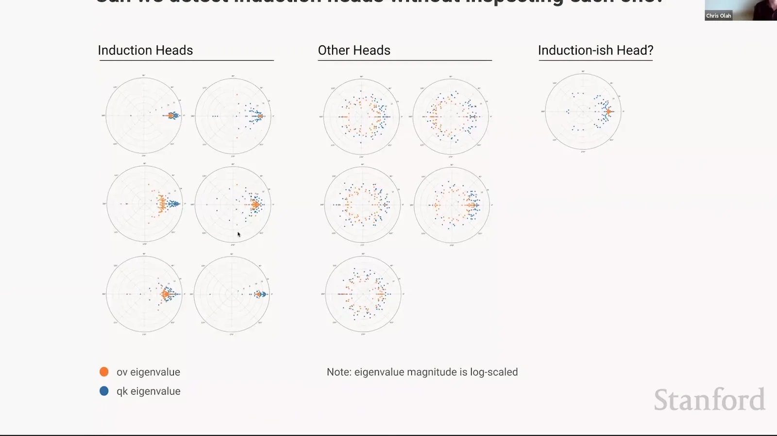
\lecturefigure{slide-52-head-taxonomy.jpg}{Induction heads、其他 heads 与 induction-ish heads 的谱/模式分类。}{Stanford Online 官方视频 00:47:30--00:47:47。}

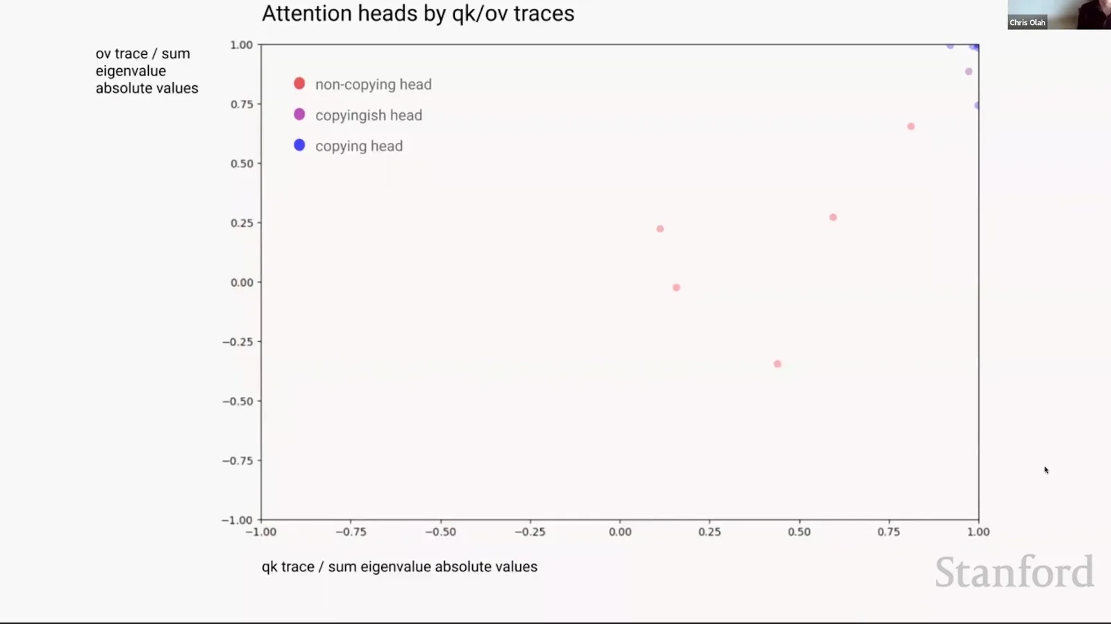
\lecturefigure{slide-53-qk-ov-trace-scatter.jpg}{QK/OV trace scatter：用两个 circuit signatures 定位 induction candidates。}{Stanford Online 官方视频 00:47:48--00:48:15。}

Signature 不是定义本身

一个 head 落在 scatter 的特定区域，只说明矩阵具有候选性质。真正 induction mechanism 还需 attention pattern、path composition、examples 与 ablation；现代模型可通过不同 basis、distributed features 或多头协作实现类似行为。

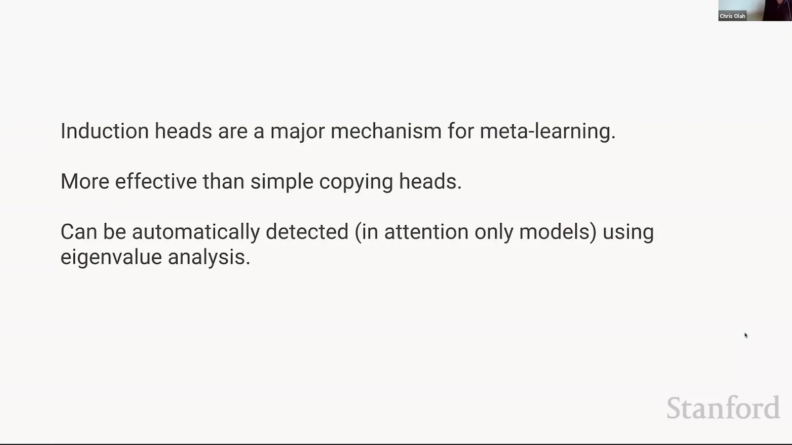
\lecturefigure{slide-54-induction-meta-learning-summary.jpg}{Induction heads 对 meta-learning 的主要贡献与自动检测思路。}{Stanford Online 官方视频 00:48:16--00:48:21。}

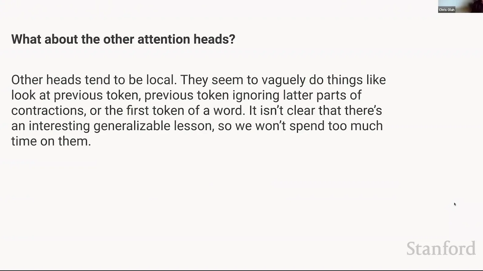
\lecturefigure{slide-55-other-local-heads.jpg}{其他 heads 往往更 local，执行 token lookup 或 position tracking。}{Stanford Online 官方视频 00:48:22--00:48:33。}

\lecturefigure{slide-56-lookup-similar-context.jpg}{Induction head 的核心：查询相似历史情境中接下来发生了什么。}{Stanford Online 官方视频 00:48:34--00:48:41。}

回到 phase-change hypothesis

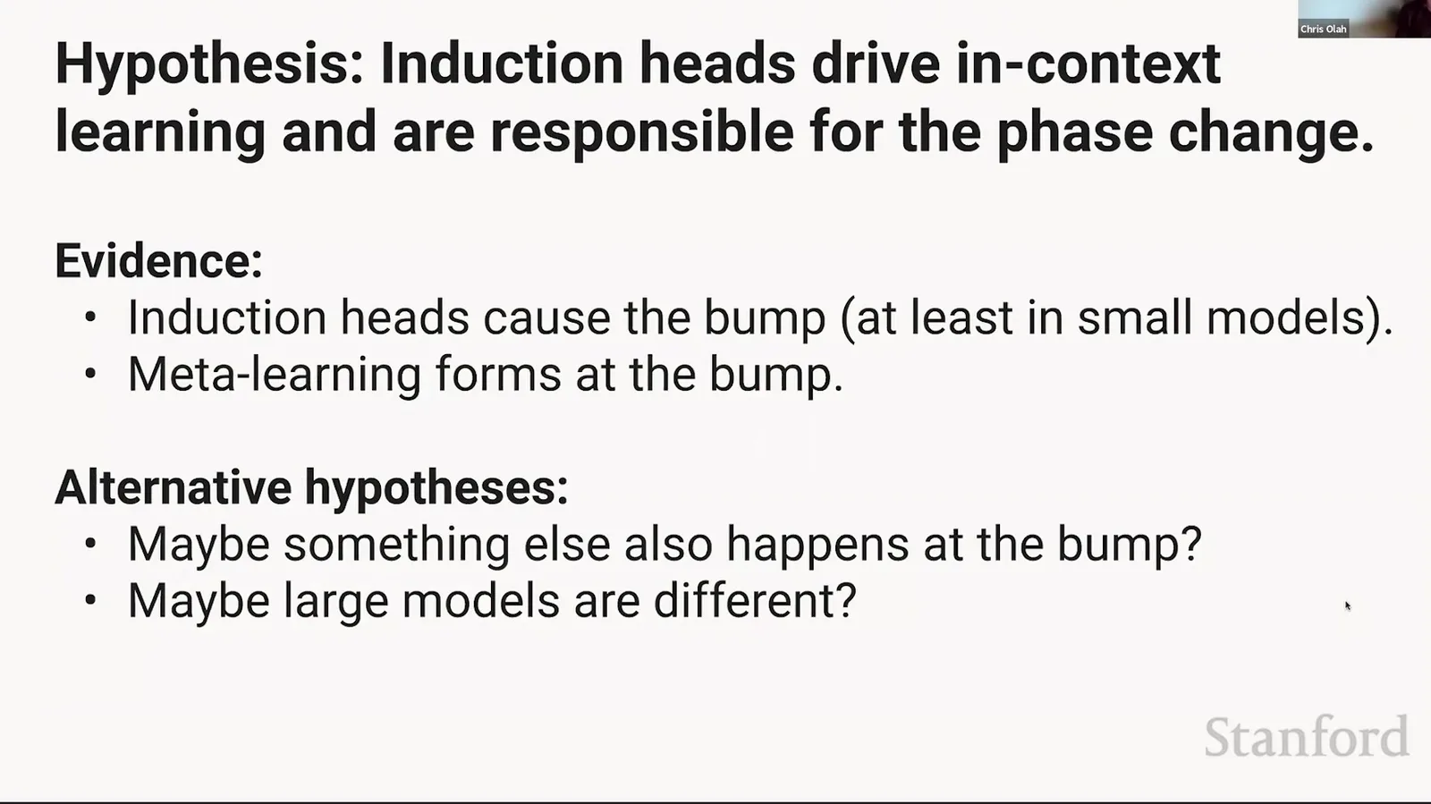
结构可行性已经具备：两层 composition 能实现 conditional lookup，induction candidates 也能从 QK/OV 与 attention pattern 中识别。于是研究假设变得具体：ICL phase change 是模型在训练中发现 induction-head circuits 的时刻。

\lecturefigure{slide-57-phase-change-hypothesis.jpg}{核心假设：induction-head 形成驱动 ICL phase change。}{Stanford Online 官方视频 00:48:42--00:49:53。}

\teachervoice{讲者再次使用 hypothesis 一词，并立即说“let's check it”。这体现了机制解释的正确节奏：先由结构提出可证伪假设，再寻找干预与跨模型证据。}

本章小结

Induction circuit 将 previous-token information 与下一层 copying head 组合成 \([A][B]\ldots[A]\to[B]\) 算法。它是可学习的 context nearest-neighbor mechanism，比无条件 copying 更精确，也给 phase change 提供了结构上可信的候选解释。

证据分级：Small-Model Causality 与 Large-Model Correlation

有了候选 circuit，最重要的问题是它是否真正驱动 measured behavior。Small attention-only models 足够简单，可以逐 head ablate 并重新计算 ICL score；large models 则更难做完整 accounting，课堂主要展示 formation timing 与 behavior timing 的重合。

Small models：直接 ablation

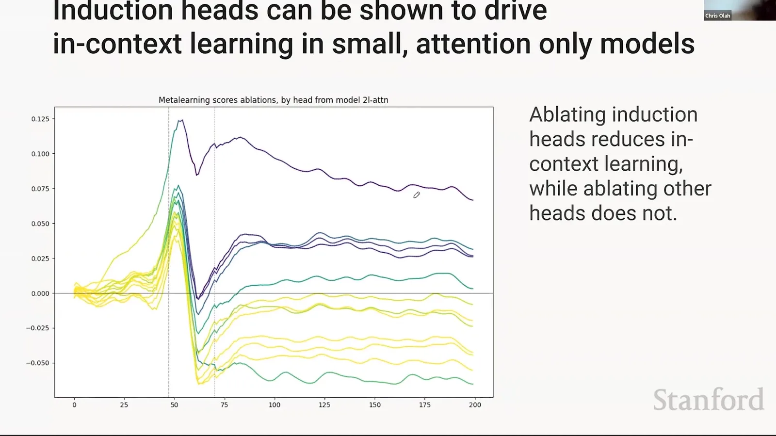
对某个 head 做 pattern-preserving ablation 或移除 contribution，比较

\[ \Delta S_h =S_{\mathrm{ICL}}^{(-h)}-S_{\mathrm{ICL}}^{(\mathrm{base})}. \]

若移除 induction head 使 score 变得不再那么负，说明 late-token advantage 被削弱。图中 head 颜色表示 induction strength，曲线表示各 head ablation 对 meta-learning/ICL score 的影响。

\lecturefigure{slide-58-small-model-ablation.jpg}{Small attention-only models：ablation 显示 induction heads 驱动 measured ICL。}{Stanford Online 官方视频 00:49:54--00:50:29。}

读图：formation dynamics 不是单调的

训练中很多 heads 一度都向 induction signature 移动，随后只有少数胜出；还有一个 induction-like head 的 ablation 方向相反。这提醒我们：head label 不是静态本体，功能会随训练竞争、冗余与 specialization 改变。

\teachervoice{Olah 对 small models 的说法最强：几乎全部 measured ICL 都可由这些 induction heads 解释。但他也指出一个 head 反向贡献，说明“像 induction”与“提高 chosen metric”并非完全等价。}

Large models：同一时间出现，但仍是 correlation

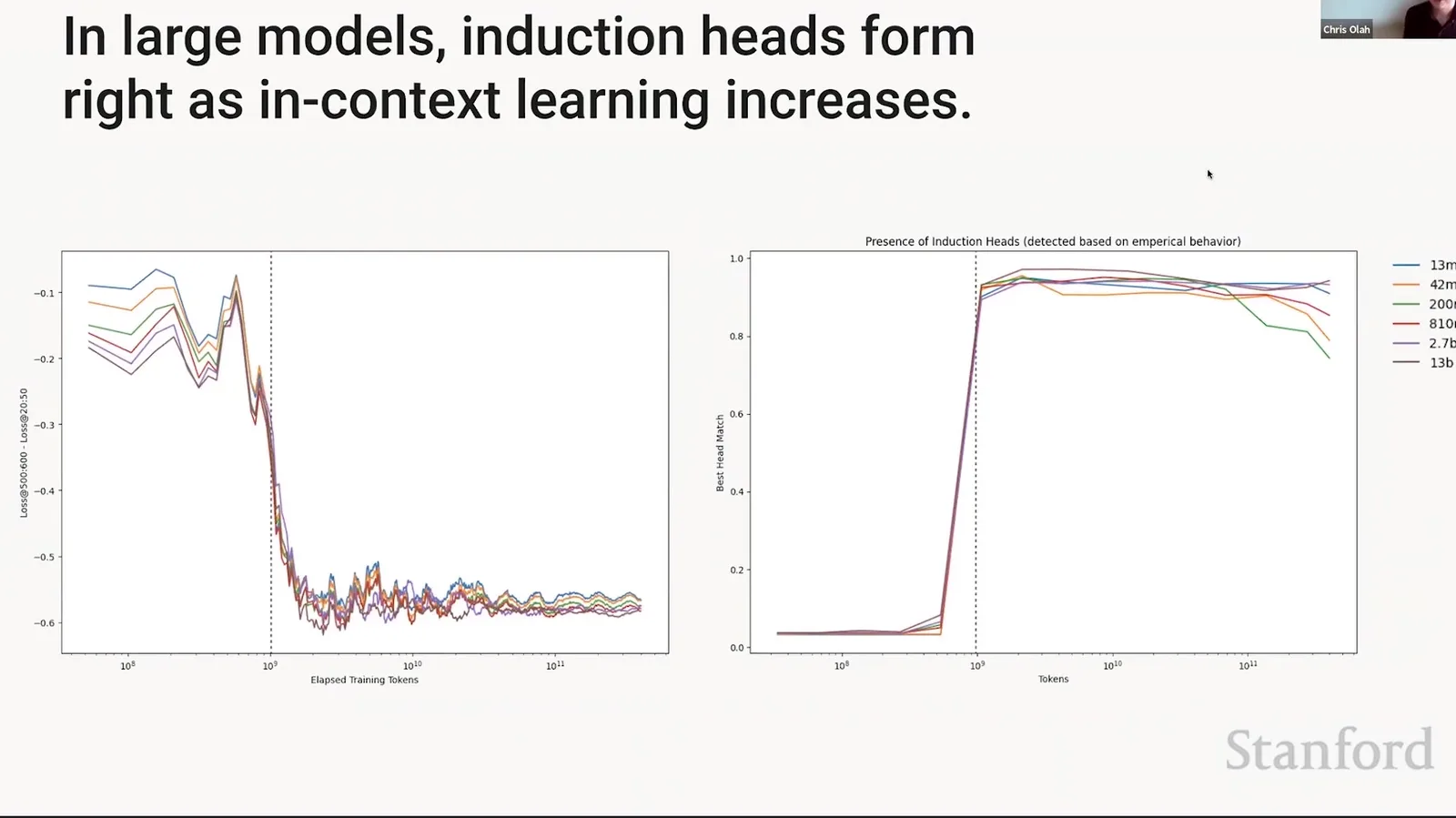
Large models 中 induction signatures 在 ICL score 快速变化的同一训练窗口形成。这个 co-occurrence 与 small-model mechanism 一致，也跨 model scales 出现，因此很有提示性；但没有同等完整的 large-model ablation accounting，仍可能有其他 circuits 同时形成。

\lecturefigure{slide-59-large-model-timing.jpg}{Large models：induction-head formation 与 ICL increase 同步。}{Stanford Online 官方视频 00:50:30--00:50:47。}

Large-model 结论必须保留“correlational”

Temporal alignment 排除了很多缓慢机制，却不能排除共同原因或同时发生的其他结构变化。课堂中 Olah 明确使用 “only correlational evidence”；讲义不能把它升级成“已经证明所有 large-model ICL 由 induction heads 引起”。

\teachervoice{讲者认为这个 correlation 很 suggestive，尤其因为 induction 具有明确 functional plausibility；但他立即补充，也可能有其他 mechanisms 在同一个窄窗口被发现。}

Generality：从 literal copy 到 translation

若 induction 只能复制完全相同的字符片段，它很难解释 richer ICL。文章与 live demo 展示 repeated chunks、cross-lingual alignment 与 analogy：例如第二句英文位置可能去读取第一句法文中对应语义后面的 token。此时 query/key 在 learned feature space 中匹配相似关系，而不是 one-hot token equality。

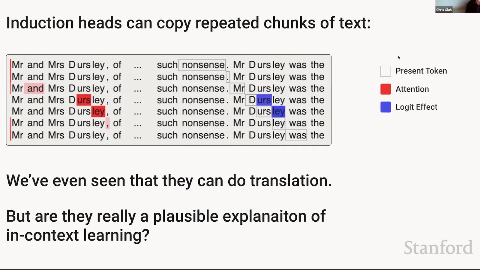
\lecturefigure{slide-60-repeated-chunk-translation.jpg}{Induction heads 可复制 chunks，并展示 translation/soft matching 行为。}{Stanford Online 官方视频 00:50:48--00:55:29。}

Soft induction

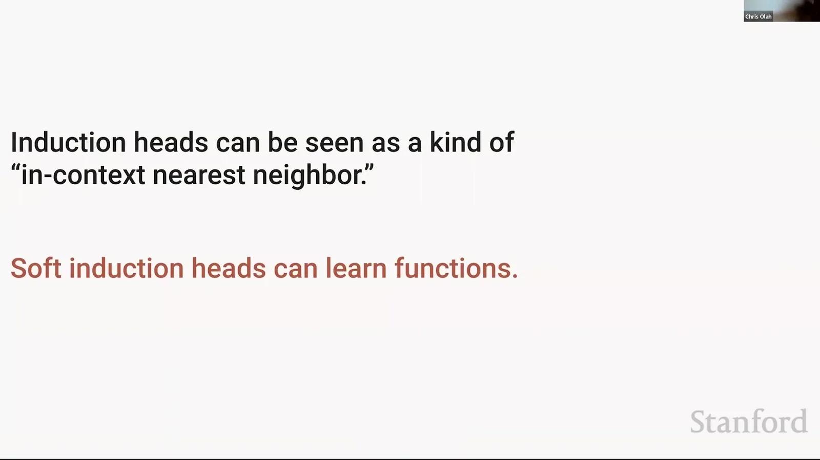
Soft induction head 学习“相似情境”的 feature match：相同 token 是特例，translation pair、同类词、格式 slot 或函数输入都可能成为 neighbors。它扩大了 induction 的解释范围，也增加了验证难度，因为相似度可能分布在多个 features 与 heads 中。

\teachervoice{Live demo 中，French/English 对应关系通过 attention 被逐步读取。Olah 把这称为 soft induction：不是原样复制 word，而是复制更抽象的 relationship 或 function。}

本章小结

Small-model ablation 给出对 ICL metric 的因果证据；large-model timing 只提供相关证据。Translation 与 soft matching 说明 induction 超越 literal copy，但也意味着机制更分布式、更难由单一 attention map 完整证明。

外推边界：其他机制、LSTM 与 Scaling Laws

Induction-head story 很有吸引力，因为它把行为、数学结构与 intervention 连在一起；越是整洁的故事，越需要主动寻找不能解释的部分。讲者在结尾明确允许其他 mechanisms，并把许多大模型计算留作开放问题。

In-context nearest neighbor 不是全部 meta-learning

Olah 将 induction 压缩为 in-context nearest neighbor，同时指出 soft heads 可以学习 functions。这个描述适合解释从 examples 中匹配和延续 pattern，却不必然覆盖 gradient-descent-like inner optimization、Bayesian updating、multi-step reasoning 或工具使用。

\lecturefigure{slide-61-in-context-nearest-neighbor.jpg}{Induction 作为 in-context nearest neighbor；soft heads 可以学习函数关系。}{Stanford Online 官方视频 00:55:30--00:55:33。}

\lecturefigure{slide-62-alternative-contributors.jpg}{其他 mechanisms 可能同时贡献 large-model ICL。}{Stanford Online 官方视频 00:55:34--00:55:59。}

漂亮的 mechanistic story 仍可能不完备

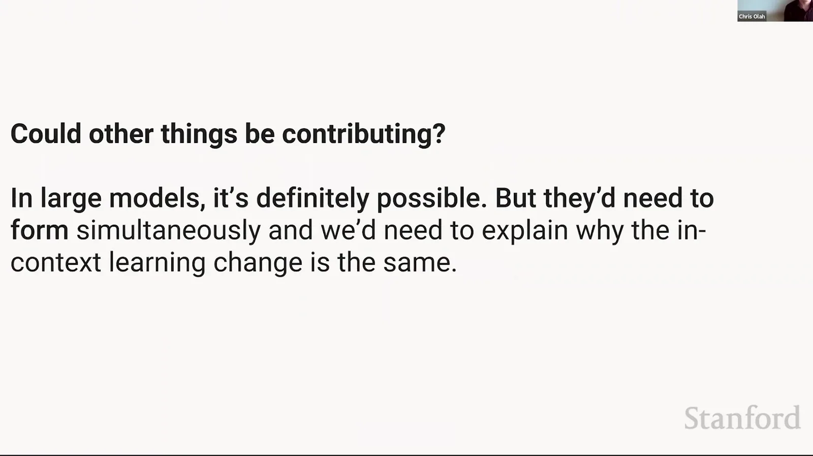
Induction heads 可以解释某类 lookup/copy behavior，并在 small models 中解释 chosen ICL score；大型模型可能同时使用 MLP memory、distributed feature binding、other heads、implicit optimization 或更长 path。最好的结论是“一个重要机制”，不是“唯一机制”。

\teachervoice{课堂结尾给出的 present theory 大致包含两类算法：一类是广泛的“看到过某词，未来合适位置可能再出现”的 copying；另一类是 induction-head nearest neighbor。讲者保留了 “possibly other things” 的空间。}

为什么 Transformer 比 bounded-state LSTM 更适合长 context lookup

Attention 可以直接访问任意过去 position，检索成本主要由 context length 与 attention implementation 决定；传统 LSTM 必须把所有历史压进固定维 recurrent state，长距离精确 lookup 容易衰减。这个差异使 induction-style retrieval 在 Transformer 中更自然，但不意味着 LSTM 数学上无法表达任何 meta-learning，也不意味着 attention 自动学到正确 lookup。

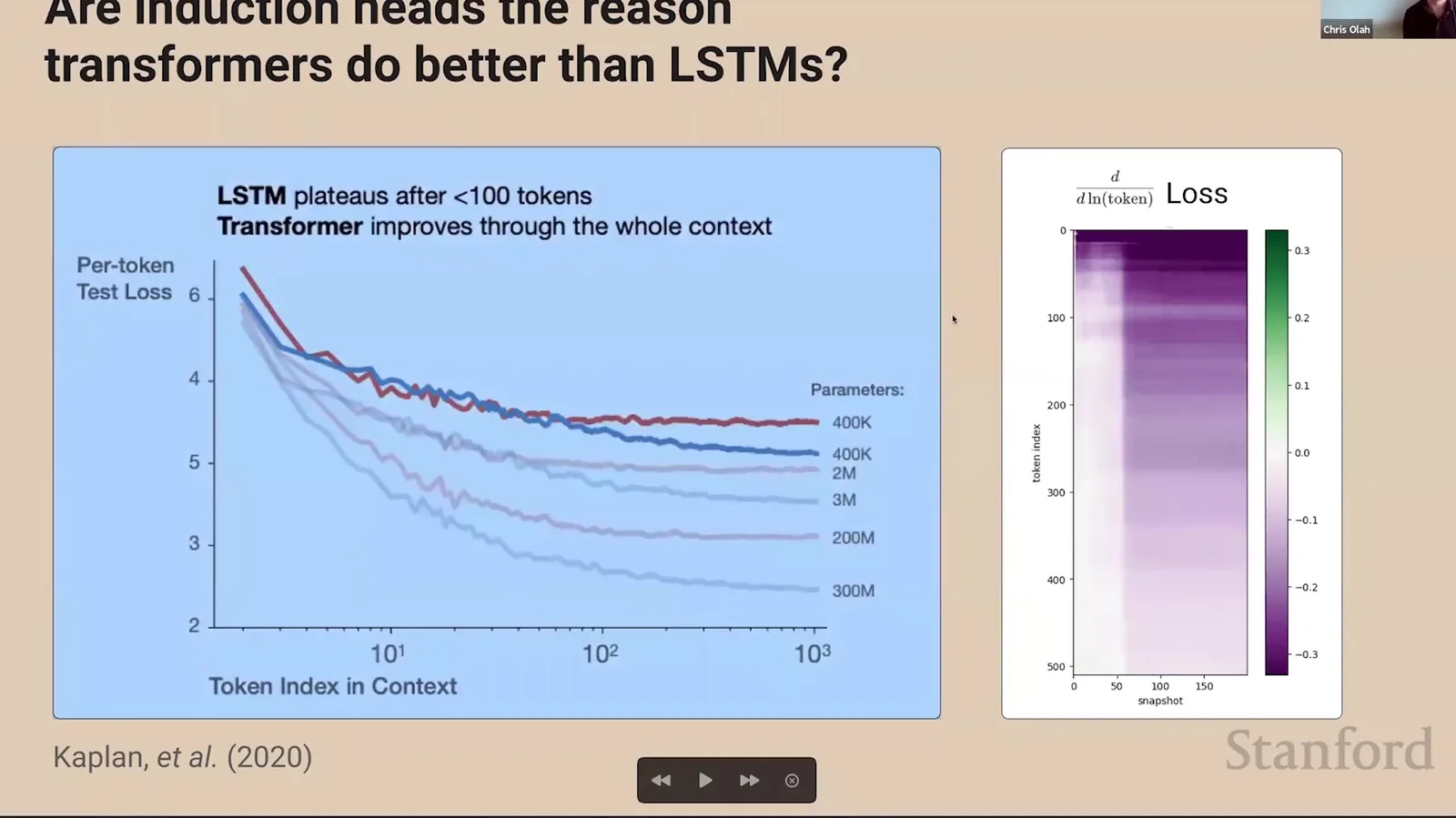
\lecturefigure{slide-63-transformer-vs-lstm.jpg}{长 context ICL：attention 的直接检索路径与 LSTM 固定状态瓶颈。}{Stanford Online 官方视频 00:56:00--00:56:21。}

不要把架构比较说成绝对不可能

有限精度、有限 hidden state 和实际训练条件下，LSTM 长距离保真 retrieval 很困难；理论上更大状态、外部 memory 或特殊训练可改变结论。课堂中的 “impossible” 应按工程语境理解为该类 mechanism 不自然、难以稳定扩展。

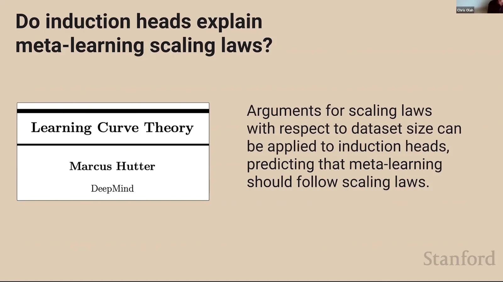
Induction heads 会解释 meta-learning scaling laws 吗

若 ICL 近似 context nearest neighbor，那么 capability 可能随 training data 中 pattern diversity、representation quality 与 context retrieval 共同变化，而不只由 parameter count 决定。讲者提出这可能帮助理解 scaling-law 曲线，但没有给出完整理论或验证。

\lecturefigure{slide-64-meta-learning-scaling-laws.jpg}{开放问题：induction-head mechanism 是否能解释 meta-learning scaling laws？}{Stanford Online 官方视频 00:56:22--00:56:47。}

\teachervoice{Olah 对 scaling-law 解释明显更 tentative：这只是可能的路线。讲义不应把一张问题页写成已建立的 law，更不能用 induction story 取代对 data distribution、optimization 与 architecture scaling 的实证分析。}

真正尚未理解的部分

Q&A 中 Olah 列出 MLP layers、arithmetic、multi-speaker/dialogue representation 与大型模型的大量内部机制。Attention-only toy models 的 near-complete account 是方法演示，不是研究终点；大模型的 nonlinear feature superposition、normalization 与 distributed circuits 仍然困难。

\teachervoice{“还有太多不了解，以至于很难回答下一步是什么”是本讲最诚实的结尾。Mechanistic interpretability 的成熟度应由可复现 circuit、干预结果与失败案例衡量，而不是由术语数量衡量。}

本章小结

Induction heads 是有结构、有 intervention 支持的重要 ICL mechanism，但大型模型可能使用其他 algorithms。Transformer 为长 context retrieval 提供自然接口，scaling-law 连接仍属开放假说，而 MLP 与 distributed circuits 是下一阶段的核心困难。

总结与延伸

从 Behavior 到 Mechanism 的完整链条

本讲最值得复用的不是某张 attention heatmap，而是一套研究程序：先定义行为指标，再寻找 abrupt change；选择可解 toy model 建立 algebra；从 path structure 提出候选 algorithm；最后用 ablation、timing、cross-example generality 与反例给证据分级。Mechanistic interpretability 的可信度来自这条链条，而不是一张“看起来像在关注正确 token”的图。

十五条核心结论

Mechanistic interpretability 尝试把 parameters 反编译为 algorithms。
ICL 固定参数，只在 context 与 activations 中发生临时适应。
二维 loss surface 同时展示 training snapshot 与 token position。
\(\mathrm{Loss@500}-\mathrm{Loss@50}\) 越负，late-context advantage 越强。
\(0.4\) nats 约为 \(0.58\) bits/token，不是 40% accuracy。
Loss bump 与 derivative spike 产生 phase-change hypothesis，但不构成证明。
Attention-only toy models 去掉 MLP/LayerNorm/bias 以换取精确 algebra。
Head 可分为 QK routing 与 OV writing 两个 circuit。
固定 attention pattern 后，attention-only path 对输入局部线性。
One-layer models 主要实现 skip-trigram/positional rules，ICL 弱且无 phase change。
Eigenvalue lens 可总结 small token-to-token maps，但在 MLP/大模型中失效。
Two-layer expansion 产生 composed/virtual heads，并允许 routing 读取前层 features。
Induction circuit 实现 \([A][B]\ldots[A]\to[B]\) 的 context nearest neighbor。
Small-model ablation 是因果证据；large-model formation timing 主要是相关证据。
Induction 是重要机制而非必然唯一机制，soft induction 与 distributed circuits 仍需更强验证。

一个可复用的 Circuit Audit Protocol

面对新的可解释性主张，可以依次检查：目标 behavior 是否量化；候选 component 是否有结构能力；路径是否跨 layers 组合；attention pattern 与 OV logit effect 是否一致；ablation 是否保留 distribution 与其他 pattern；结果是否跨 prompts/seeds/models；结论是否区分 toy model、small model 与 production-scale model。

实践检查表

定义 behavior metric 与 sign convention；
画 training × context 的二维诊断，而非只看最终 checkpoint；
展开 residual paths，区分 routing 与 writing；
用 activation/attention 找 hypothesis，用 ablation 做因果检查；
记录 compensation、redundancy 与 negative-result heads；
对 large-model extrapolation 标注 correlation、plausibility 或 intervention；
主动寻找 alternative mechanism 和 failure case。

拓展阅读

建议先读 A Mathematical Framework for Transformer Circuits 的 one-/two-layer decomposition，再读 In-context Learning and Induction Heads 的 evidence taxonomy 与 appendix。随后对照 Kaplan scaling laws 和 GPT-3 few-shot behavior，思考 behavioral curve、training dynamics 与 circuit formation 的关系。阅读现代大型模型解释工作时，应重点观察它们如何处理 MLP nonlinearities、feature superposition、normalization、distributed computation 与 causal validation，而不是只比较 head visualizations 是否漂亮。

\teachervoice{本讲最后的 present theory 是两个主要 algorithms：广义 copying 与 induction-head in-context nearest neighbors，同时承认可能还有别的机制。把这份不确定性保留下来，正是对课堂与原始研究最忠实的总结。}