Lecture29

LaTeX 源码

\makecscover

讲座定位：理解 Mixtral 要同时记三本账

Mixtral 常被压缩成一句话：“八个 7B 专家，每个 token 只激活两个。”这句话足够吸引注意，却不足以解释模型为什么快、为什么占显存、为什么需要复杂通信，也不足以说明所谓“专家”究竟学到了什么。本讲的正确入口是同时维护三本账：总容量记录所有专家能存下多少参数，活跃计算记录一个 token 实际经过多少参数，系统成本记录权重驻留、token dispatch、跨卡通信和负载不均衡。三者不能相互替代。

先修复来源，再建立阅读路线

本节先说明材料边界，因为旧目录存在严重来源污染：旧幻灯片文件实际是 Nathan Lambert 的 Lecture 28 对齐课程 deck，并非 Albert Jiang 的 Mixtral 讲座。CS25 官网没有给本讲发布独立 deck，因此本讲从官方 1920x1080 录像逐秒恢复 slide states，并把 34 分钟 Q&A 作为 teacher voice 融入正文。接下来的图都来自官方录像，而不是错误 PDF。

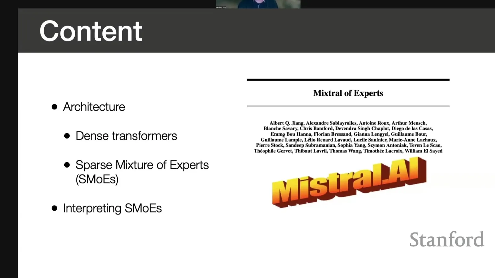
\lecturefigure{slide-01-content.jpg}{课程路线：dense Transformer、Sparse Mixture of Experts 与 routing interpretation}{Stanford Online 官方录像 00:01:59}

本讲的核心问题

Sparse Mixture of Experts（SMoE，稀疏专家混合）不是“更大的 dense model”。它把每层的单个 MLP 扩成多个 expert MLP，再由 router 为每个 token 选择少量专家。这样可以提高总容量而不同比例提高每 token FLOPs；但所有专家仍需存储，token 仍需在设备间移动，router 仍可能把负载压到少数专家。

术语消化：三本账分别回答什么

账本	核心问题	典型变量
总容量	模型一共存了多少权重？	total parameters、所有 experts、shared attention
活跃计算	一个 token 实际经过哪些权重？	top-\(k\)、active parameters、per-token FLOPs
系统成本	权重和 token 怎样落在硬件上？	HBM（High Bandwidth Memory，高带宽显存 DRAM）、expert parallelism、all-to-all、batch、load balance

\teachervoice{00:01:04--00:01:54，Albert 把课程明确分成 architecture 与 interpretation 两部分，并反复插入 open research questions。他希望开放社区继续研究，而不是把 Mixtral 当成已经解释完的配方。}

证据等级：哪些是测量，哪些只是工作假设

这堂课同时包含模型配置、benchmark plot、routing histogram、社区 ablation 和 Q&A 经验判断。阅读时必须区分：模型参数表是结构事实；2024 年 benchmark 是当时的比较证据；“MLP 存知识、attention 做推理”是 speaker 明说的 conventional wisdom；某个 expert 在数学数据上被多选只是相关性；“更大 expert count 更易专门化”则是前瞻判断。后文会在每一处标出边界。

名字里的 expert 不等于人类职业专家

Expert 只是可被 router 选择的参数子网络。它可能对 token 形态、局部语法、位置、频率或多个潜在特征的线性组合敏感，并不天然对应“代码专家”“医学专家”。把 router 选择直接翻译成人类语义，是本讲要纠正的第四个 myth。

本章小结

本讲的教学主线不是模型宣传，而是把 sparse capacity、active compute、resident memory、communication 与 interpretability 放进同一系统。来源修复也意味着：所有 slide coverage 和教师口头解释必须重新建立，旧讲义不能沿用。

Dense baseline：先看 Mistral 7B 如何组织 attention 与 MLP

Mixtral 并没有重写整个 Transformer。它沿用 Mistral 7B 的 attention 与 residual structure，只把每层 MLP 换成 top-two-of-eight expert MLP。为了准确理解“只改了哪里”，本章先建立 dense baseline：Grouped-Query Attention、Sliding-Window Attention、RMSNorm、SwiGLU 与 tensor shape。

MHA、MQA 与 GQA：先数 query head 和 KV head

标准 Multi-Head Attention（MHA）让每个 query head 都有独立 key/value head；Multi-Query Attention（MQA）让所有 query heads 共享一组 K/V；Grouped-Query Attention（GQA）位于两者之间，让一组 query heads 共享一个 KV head。Mistral 7B 使用 32 个 query heads 和 8 个 KV heads，目标是保留更多表示自由度，同时降低 KV cache 和 memory bandwidth 压力。

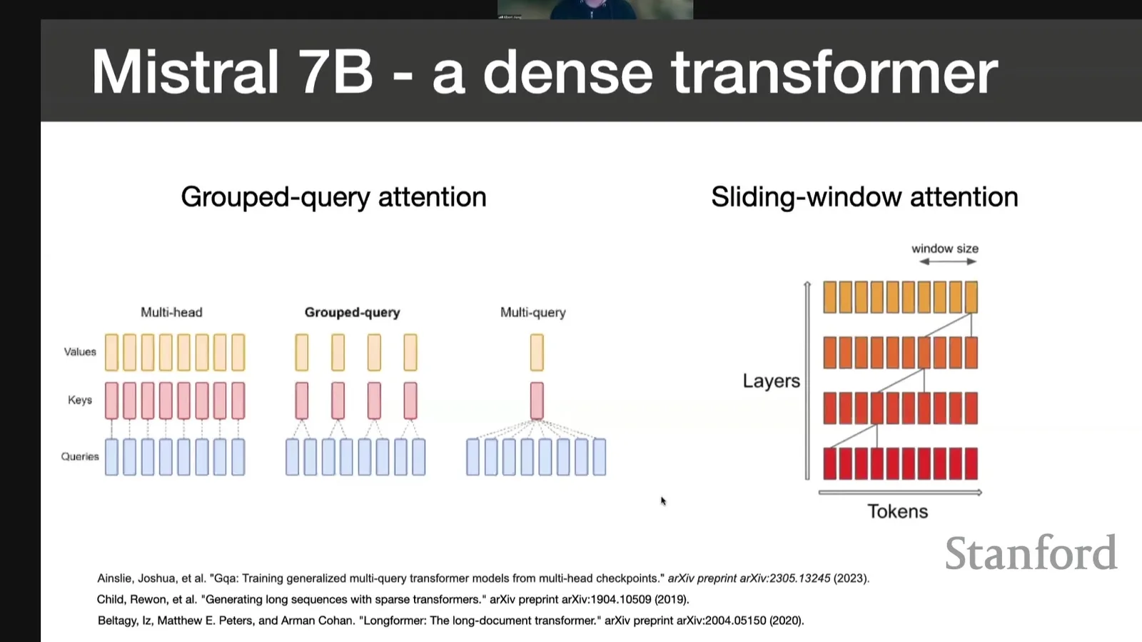
\lecturefigure{slide-02-dense-attention.jpg}{Mistral 7B 的 Grouped-Query Attention 与 Sliding-Window Attention}{Stanford Online 官方录像 00:03:55}

设 query head 数为 \(H_q\)，KV head 数为 \(H_{kv}\)，head dimension 为 \(d_h\)，序列长度为 \(L\)。自回归解码时，每层 KV cache 的元素量近似为

\[ N_{KV}=2L H_{kv}d_h, \]

其中系数 \(2\) 对应 key 与 value。若从 MHA 的 \(H_{kv}=H_q=32\) 改成 GQA 的 \(H_{kv}=8\)，同精度、同序列长度下 KV cache 约降为四分之一。

Attention 的核心仍是

\[ \operatorname{Attn}(Q,K,V)=\operatorname{softmax}\!\left(\frac{QK^{\top}}{\sqrt{d_h}}+M\right)V, \]

其中 \(M\) 是 causal/sliding-window mask。GQA 改的是 K/V 的共享方式，不是这条概率加权公式本身。

背景概念：KV cache 为什么是推理成本

KV cache 保存过去 token 在每层生成的 key/value，避免每次解码重新计算全部前缀。它主要驻留在 GPU 的 HBM（High Bandwidth Memory，高带宽显存 DRAM）中；长度、层数、KV head 数或 batch 增长都会线性增加容量，并消耗读写带宽。因此 GQA 的收益不仅是“少几个矩阵”，而是减少长期驻留状态。

GQA 不等于免费压缩

减少 KV heads 可能损失不同 query heads 对 K/V 表示的独立性。最终质量取决于模型规模、训练数据和 head grouping；不能只由缓存公式推导 benchmark 结果。

\teachervoice{00:02:18--00:03:36，Albert 强调 GQA 与 sliding-window attention 都不是 Mistral 新发明，而是把已有设计组合进一个强 dense baseline。课程关注的是工程选择如何共同工作，而非抢单点 novelty。}

Sliding-window attention：局部窗口如何跨层传播

GQA 解决 KV head 数，Sliding-Window Attention（SWA，滑动窗口注意力）解决单层可见范围。每个位置只直接注意最近 \(w\) 个 token，因此单层 attention matrix 从全局 \(L^2\) 连接缩到约 \(Lw\)；但信息可沿层数逐步传播，所以深层 token 能间接吸收更远上下文。

可把第 \(\ell\) 层位置 \(t\) 的直接可见集合写成

\[ \mathcal{N}_{\ell}(t)=\{j\mid \max(0,t-w+1)\le j\le t\}. \]

若每层都允许局部传递，理想化的最大信息传播距离随层数增长，约为 \(\ell(w-1)\)。这不是“第 \(\ell\) 层拥有无损全局 attention”的证明，但说明局部计算可以通过 depth 扩散。

GQA 与 SWA 解决不同瓶颈

GQA 主要降低 K/V 表示和 KV cache；SWA 主要减少每层 attention 连接和长序列计算。两者可以同时使用，因为一个改 head sharing，一个改 token neighborhood。

一层 dense Transformer：读 shape 比背模块名更可靠

架构图容易隐藏细节，因此讲者直接给出一个单层 PyTorch 实现，并把 tensor dimension 写进变量名。读代码时应跟踪四件事：Q/K/V projection 的 shape、RoPE 后的位置编码、attention residual、SwiGLU MLP residual。这样才能看到 Mixtral 后面真正替换的只有 MLP 路径。

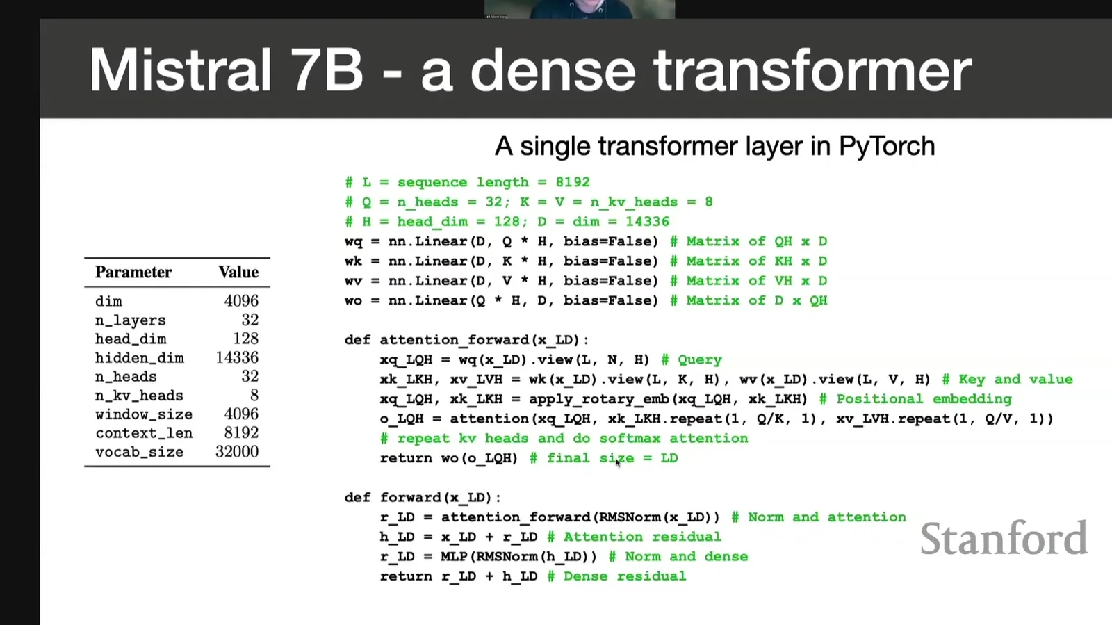
\lecturefigure{slide-03-dense-layer-code.jpg}{Mistral 7B 单层 Transformer 的参数表与 PyTorch 实现}{Stanford Online 官方录像 00:06:45}

若输入 \(X\in\mathbb{R}^{L\times d}\)，dense block 可概括为

\[ \begin{align} H &= X+\operatorname{Attention}(\operatorname{RMSNorm}(X)),\\ Y &= H+\operatorname{MLP}(\operatorname{RMSNorm}(H)). \end{align} \]

Mistral 使用 SwiGLU 风格 MLP，可写为

\[ \operatorname{MLP}(x)=W_2\left(\operatorname{SiLU}(W_1x)\odot W_3x\right), \]

其中 \(W_1,W_3\) 把 hidden dimension 扩到 intermediate dimension，\(W_2\) 再投影回来，\(\odot\) 是逐元素乘法。Mixtral 的 expert 就是复制这种 MLP 参数化，而不是复制整层 attention。

Dense Transformer block 的 shape-first 伪代码

q = x @ Wq            # [tokens, query_heads, head_dim]
k = x @ Wk            # [tokens, kv_heads, head_dim]
v = x @ Wv            # [tokens, kv_heads, head_dim]
h = x + attention(q, k, v, causal_window)
y = h + swiglu(rms_norm(h), W1, W2, W3)

首次使用：fused kernel

Fused kernel（融合 kernel）把 RMSNorm、projection、activation 或 gating 等多个 GPU 操作合并成更少的 kernel launch，减少 HBM 中间结果读写与 launch overhead。它能改善真实吞吐，但不会改变模型数学结构，因此不能用 kernel 优化掩盖 total/active parameter 的概念差异。

\teachervoice{00:03:36--00:06:49，讲者说 Transformer architecture 有大量细小 decision choices，仅放一张框图不够，所以用带 tensor-shape 后缀的代码告诉听众每个矩阵到底做什么。}

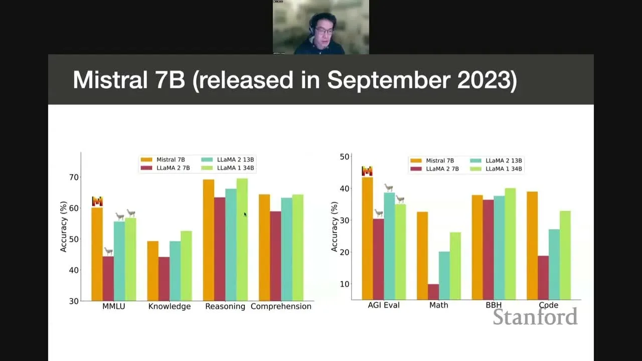
Dense baseline 的证据：小模型不等于弱模型

在进入稀疏模型前，课程用 Mistral 7B 的当时 benchmark 说明 dense baseline 已经很强。图中的比较是 2023 年发布时的模型快照，不是 2026 年 leaderboard；它的作用是控制变量：Mixtral 的增益必须相对同家族 Mistral 7B 理解，而不是把所有改进都归因于 MoE。

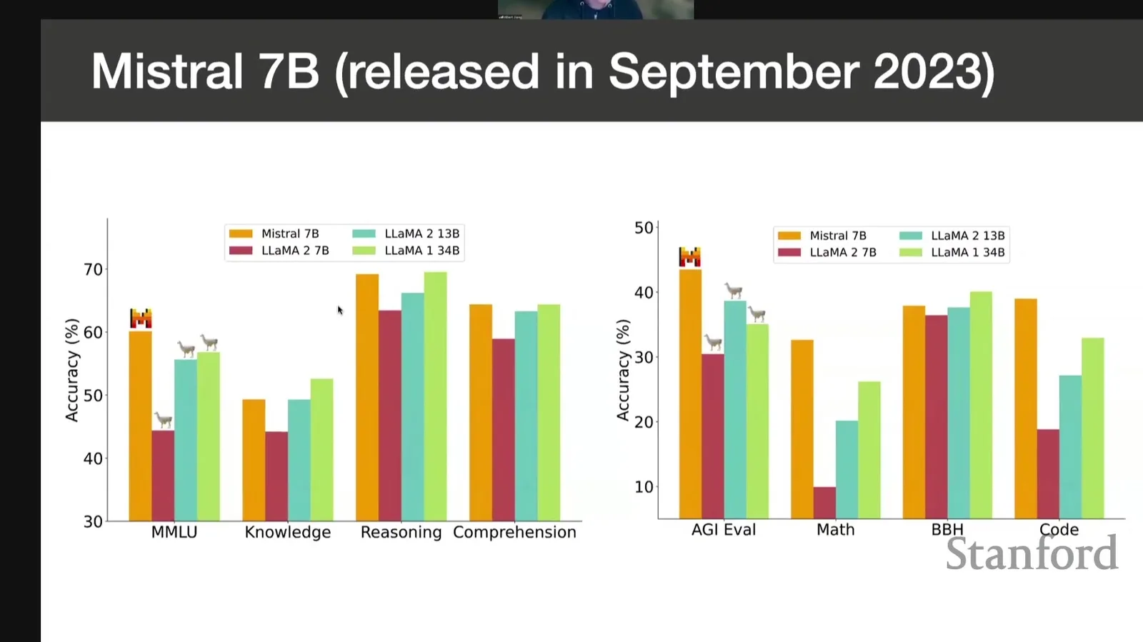
\lecturefigure{slide-04-mistral7b-performance.jpg}{Mistral 7B 在 2023 年发布时的 benchmark 比较}{Stanford Online 官方录像 00:07:01}

读图：先确认模型大小，再看任务类别

图把 Mistral 7B 与多种 Llama 2 配置比较。第一步不是寻找最高柱，而是确认每个 baseline 的参数规模；第二步看不同任务是否一致；第三步检查是否存在只在单个 benchmark 上的优势。课程只用它证明 dense baseline 有竞争力，不把任何柱状图当作通用能力排名。

历史 benchmark 的可比性边界

Prompt、few-shot 设置、tokenizer、evaluation harness 和 contamination 都可能改变分数。这里的图用于解释为什么团队从 Mistral 7B 出发研究 Mixtral，而不用于与更新模型横向比较。

本章小结

Mistral 7B 提供了清晰的 dense control：GQA 减少 KV heads，SWA 限制单层连接，RMSNorm/SwiGLU 组织 residual block。Mixtral 保留这些结构，把第二条 residual branch 的单个 MLP 替换成 sparse expert mixture。因此后面的容量与成本分析都应以“共享 attention + 多个 expert MLP”为基础。

Sparse MoE mechanism：router 如何选择并组合 experts

上一章确认了被替换的对象是 MLP，本章进入真正的 SMoE 机制。关键不是简单复制八份网络，而是建立 token-to-expert routing：router 为每个 token 产生 score，选 top-\(k\)，对选中 score 归一化，再把多个 expert 输出加权求和。整个过程需要可微、可并行、可平衡。

MoE 不是新概念：从 sparsely-gated layer 到 Switch Transformer

课程先展示文献脉络，提醒读者不要把 Mixtral 的成功误认为 MoE 概念首次出现。2017 年的稀疏门控 MoE 已用 gating network 选择子网络；Switch Transformer 进一步讨论 data/model/expert parallelism 与大规模稀疏训练。Mixtral 则把这些思想放进开放权重的高质量 decoder-only 模型，并给出可分析的 routing evidence。

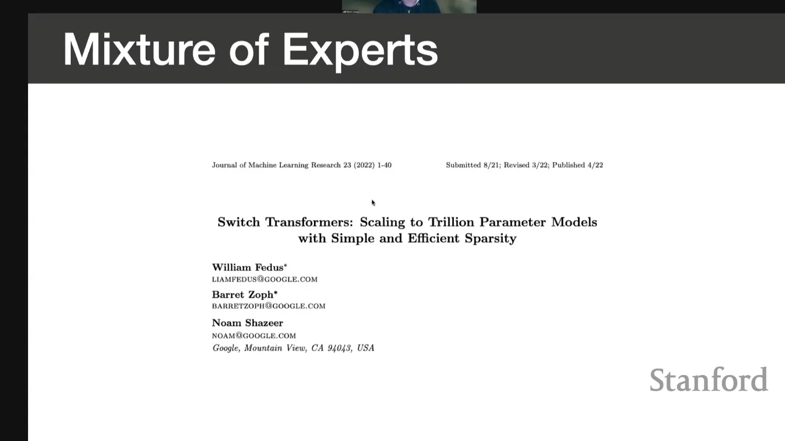
\lecturefigure{slide-05-moe-history.jpg}{Mixture of Experts 的历史参考：稀疏门控与 Switch Transformer}{Stanford Online 官方录像 00:07:49}

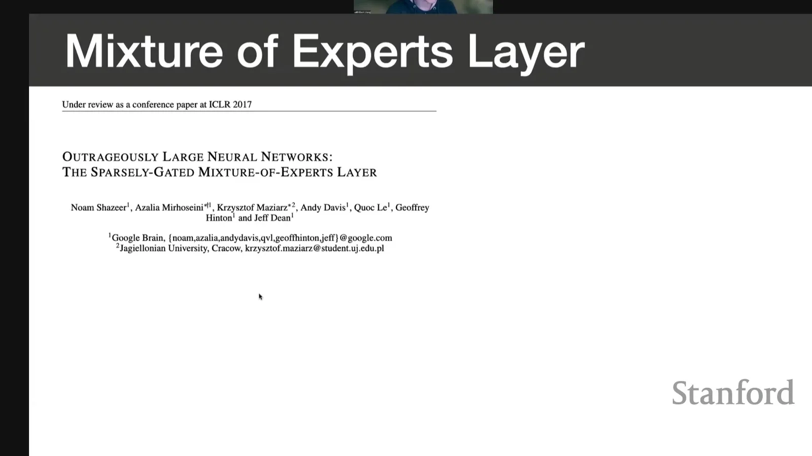
\lecturefigure{slide-06-moe-layer-references.jpg}{Sparse MoE layer 的直接文献来源}{Stanford Online 官方录像 00:08:02}

术语消化：parallelism 不只是“多卡”

方式	分割对象	主要通信
Data parallelism	不同 batch shards，模型复制	gradient all-reduce
Tensor/model parallelism	单层矩阵或 hidden dimension	all-reduce / all-gather
Expert parallelism	不同 experts 放在不同 ranks	token all-to-all dispatch / combine
Pipeline parallelism	不同层放在不同 stages	activation send/receive

Collectives 是多 GPU 集合通信原语，例如 all-reduce、all-gather、reduce-scatter 和 all-to-all。MoE 最有代表性的通信是 all-to-all：每张卡把 token 发给拥有目标 expert 的卡，计算后再把结果送回。

\teachervoice{00:07:01--00:08:24，Albert 反复说 MoE “not new”。他特别推荐 Switch Transformer 的 parallelism 讨论，并把 Mixtral 放进 2017 年 sparsely-gated layer 的连续谱系。}

Top-two routing：从 logits 到 weighted expert output

对一个 token representation \(x\in\mathbb{R}^{d}\)，router 用矩阵 \(W_r\in\mathbb{R}^{E\times d}\) 产生 \(E\) 个 expert logits：

\[ z=W_rx. \]

设 \(S_k(x)\) 是 \(z\) 最大的 \(k\) 个 expert index，Mixtral 使用 \(E=8,k=2\)。只在选中集合上归一化：

\[ g_i(x)= \begin{cases} \dfrac{\exp(z_i)}{\sum_{j\in S_k(x)}\exp(z_j)}, & i\in S_k(x),\\[0.8em] 0, & \text{otherwise}. \end{cases} \]

最终 MoE MLP 输出为

\[ y=\sum_{i=1}^{E}g_i(x)\,\operatorname{Expert}_i(x). \]

这三步分别回答“打分”“选择”“组合”。Sparse 的含义是只有 \(k\) 个 expert 执行，而不是其余权重从模型中消失。

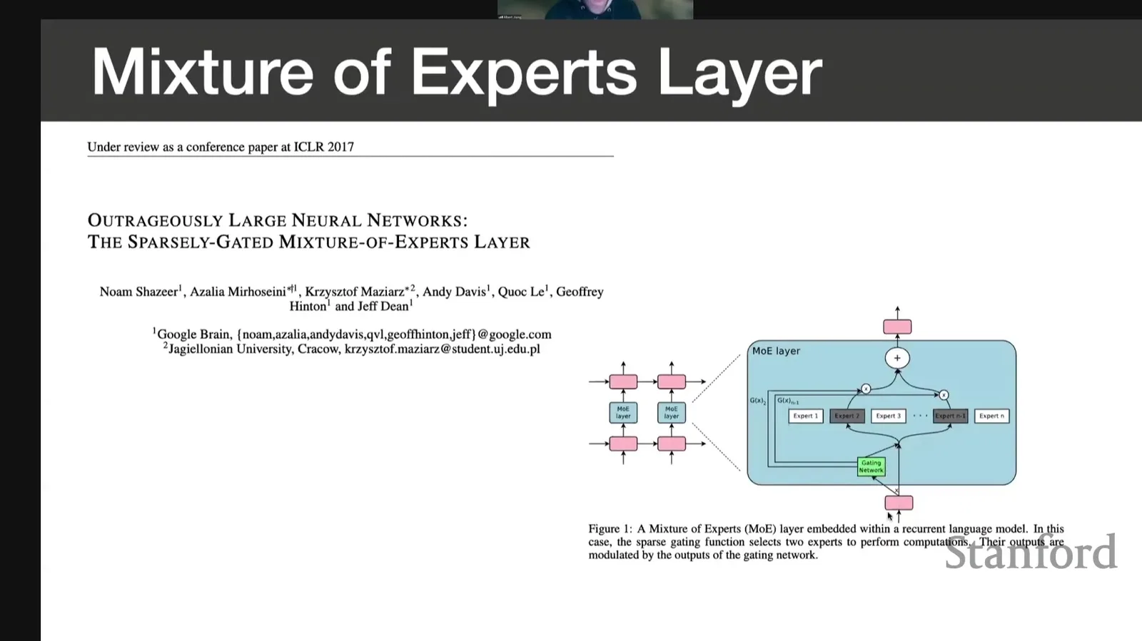
\lecturefigure{slide-07-moe-layer-diagram.jpg}{Router 为每个 token 选择 experts 并合并输出}{Stanford Online 官方录像 00:08:19}

Top-\(k\) routing 的算法语义

每个 token 独立路由；同一序列相邻 token 可以选择不同 experts；同一个 expert 会同时接收来自许多序列的 token。实现必须把 token 按 expert 重新排列、跨卡 dispatch、批量执行 expert MLP，再 inverse-permute 回原顺序。

Top-two token routing 的最小伪代码

router_logits = hidden @ router_weight.T
expert_ids = topk(router_logits, k=2)
gates = softmax(gather(router_logits, expert_ids), dim=-1)
expert_inputs = dispatch_by_expert(hidden, expert_ids)
expert_outputs = run_selected_experts(expert_inputs)
output = combine_and_restore_order(expert_outputs, gates)

\teachervoice{00:08:24--00:09:18，讲者按同样顺序口头拆解：input 先进入 router，router 选 top two 并给 gating weights，各 expert 独立处理，再用 weights 加权求和。}

公式页与参数表：读出 \(E=8\)、\(k=2\)E=8、k=2 和 shared parts

公式页把机制和模型配置放在同一张 slide 上。读表时要把 num_experts=8 与 top_k_experts=2 分开：前者决定每层可用容量，后者决定一个 token 的活跃路径。Attention、embedding、router 和 residual structure 是 shared parameters，不随 expert 数简单乘八。

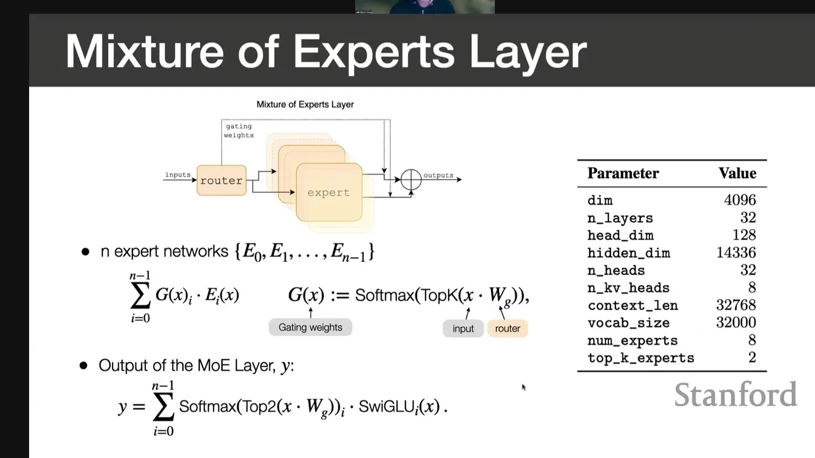
\lecturefigure{slide-08-moe-equation-table.jpg}{Mixtral 的 top-two routing 公式与模型参数表}{Stanford Online 官方录像 00:09:27}

把每层 shared parameter 记为 \(P_s\)，单个 expert MLP 参数记为 \(P_e\)，层数为 \(N\)，则粗略的总参数与活跃参数为

\[ \begin{align} P_{\text{total}} &\approx P_{\text{embed}}+N(P_s+E P_e),\\ P_{\text{active}} &\approx P_{\text{embed}}+N(P_s+k P_e). \end{align} \]

因此模型名中的 \(8\times 7\mathrm{B}\) 既不是精确总参数，也不是每 token 激活参数；shared parts 使简单乘法失真。

“稀疏”发生在执行路径，不发生在存储存在性

未选中的 expert 在当前 token 上不执行，但它们仍属于 checkpoint，通常仍需驻留在 GPU HBM、CPU DRAM 或其他层级。Resident memory 由 total parameters 决定，per-token MLP FLOPs 更接近 active parameters 决定。

Mixtral 8x7B：容量与活跃路径的正式合流

现在可以读完整模型 slide。Mixtral 继承 Mistral 7B 的 attention block，每层有八个 SwiGLU experts，每个 token 选两个。课程给出的 release-time 数字约为 46.7B total parameters 与 12.9B active parameters；它们分别对应容量/驻留与每 token 执行路径，不能互换。

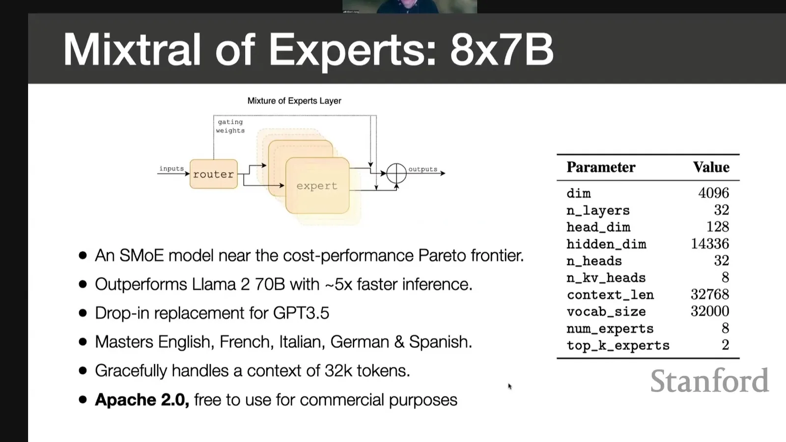
\lecturefigure{slide-09-mixtral-8x7b.jpg}{Mixtral 8x7B 的模型结构、参数表与发布时能力摘要}{Stanford Online 官方录像 00:10:26}

Mixtral 的一句准确描述

Mixtral 8x7B 是“共享 attention 与路由器、每层八个 expert MLP、每 token top-two 激活”的 decoder-only SMoE。它不是八个独立 7B 模型投票，也不是只占 13B 权重内存的 dense model。

\teachervoice{00:09:38--00:10:17，Albert 用 active path 解释 cost-performance frontier，同时列出当时的多语言、32K context、Apache 2.0 与 benchmark claim。讲义把这些保留为 2024 年 release-time 证据，不当作当前产品规格。}

本章小结

Sparse MoE 的数学结构很短：router logits、top-\(k\) mask、selected softmax、expert weighted sum；真正困难的是把这条 token-level 算法放到多 GPU 上并保持负载均衡。总参数与活跃参数的分解，是后面所有 myth、性能和部署讨论的共同基础。

为什么 MoE-fy MLP：性能证据与工作假设

上一章解释“怎样路由”，本章追问“为什么优先扩 MLP”。讲者采用一个常见但未证明的分工直觉：MLP 更像知识存储，attention 更像组合与算法。若这个直觉有部分成立，扩大 MLP capacity 应对 knowledge-heavy tasks 更有帮助；课程随后用两组 benchmark 图检验这种趋势，并提出 MoE-fying attention 的反问题。

MLP 存知识、attention 做算法：有用但危险的直觉

这张 slide 的价值在于明确写出假设，而不是证明假设。Transformer 的知识和计算分布在 embeddings、attention、MLP、normalization 与 residual interactions 中；把功能二分可以组织实验，但不能据此断言某个 layer 或 expert 只负责一种认知功能。

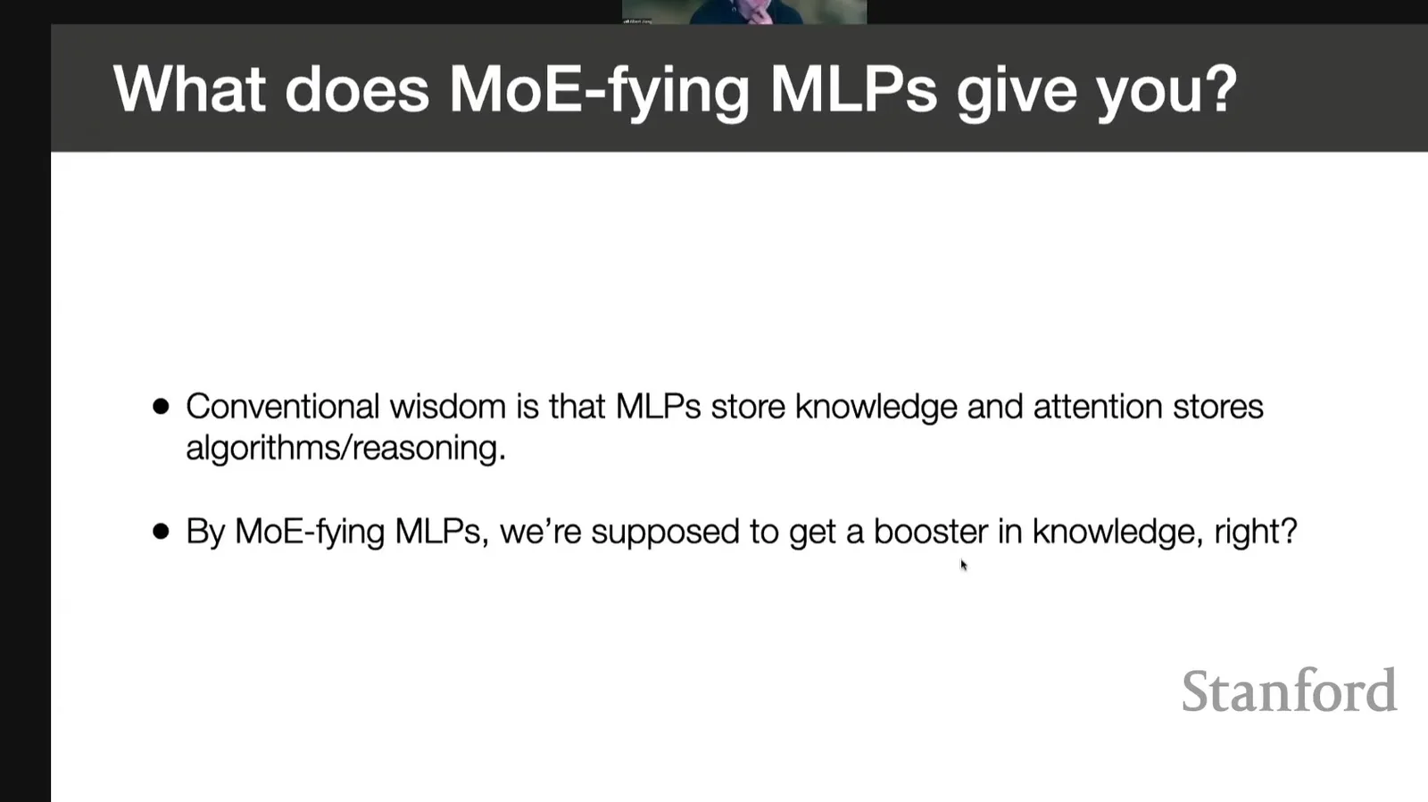
\lecturefigure{slide-10-why-moe-mlp.jpg}{为什么优先 MoE-fy MLP：knowledge-versus-reasoning 的工作假设}{Stanford Online 官方录像 00:10:58}

不要把机制直觉写成定位定理

即使 MLP 扩容与 knowledge benchmark 同时提升，也不能推出“知识只存在 MLP”。参数更多、训练动态变化、router regularization 和数据利用都可能影响结果。可靠表述应是：本讲用该直觉提出预测，再看任务类别是否大致符合。

\teachervoice{00:10:32--00:11:44，Albert 直接称这一区分为 conventional wisdom，并预期 MoE-fying MLP 最明显地提高 knowledge；他没有把它包装成严格神经科学结论。}

Category bars：知识任务增益最大，但不是唯一增益

柱状图比较 Mistral 7B、Mixtral 8x7B 与若干 Llama 2 baselines。读图时先按 category 分组，再比较同家族 dense/sparse 差值；不要先看总平均。讲者观察到 knowledge-heavy tasks 的提升最明显，reasoning/comprehension 也有提升但幅度较小。

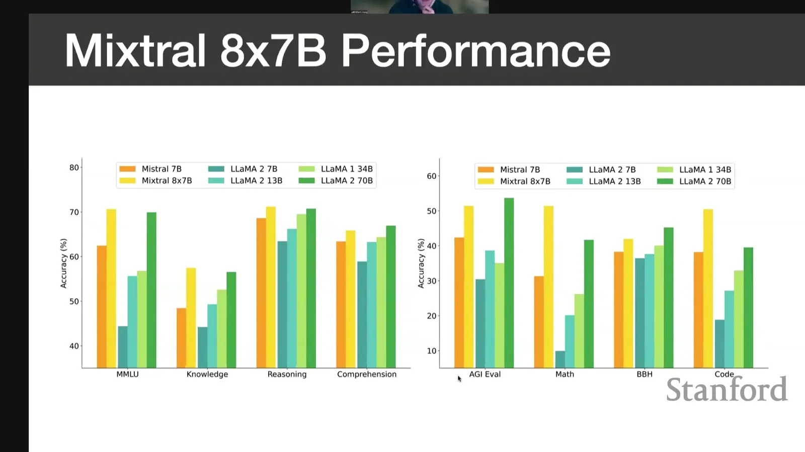
\lecturefigure{slide-11-mixtral-performance-bars.jpg}{Mixtral 8x7B 在不同任务类别上的 release-time benchmark}{Stanford Online 官方录像 00:11:41}

若某任务分数为 \(s_m\)，同 baseline 分数为 \(s_b\)，可用相对增益

\[ \Delta_{\mathrm{rel}}=\frac{s_m-s_b}{|s_b|+\epsilon} \]

比较不同量纲，但它仍不解决 benchmark saturation、prompt sensitivity 或 contamination。图的教学结论是“增益分布不均”，而不是“知识与推理已被完全分离”。

读图：四步避免 category cherry-picking

第一，确认每组是否使用同一 evaluation harness；第二，区分 accuracy、exact match 等 metric；第三，看同家族 Mistral 7B 到 Mixtral 的差值；第四，再看是否跨类别一致。只挑最大柱会夸大 MoE 的普适性。

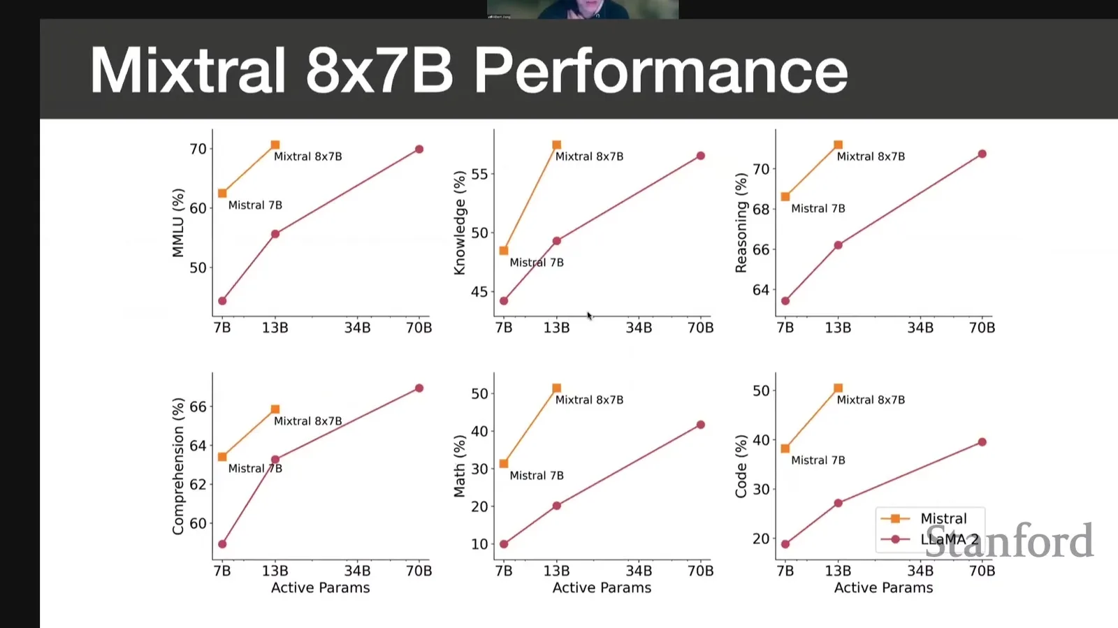
Active-parameter plot：横轴不是 total model size

第二组图把横轴设为 active parameters，强调 Mixtral 每 token 约使用 12.9B 参数，却处在更优 performance region。这个坐标回答“相近活跃计算得到多少质量”，并不回答“checkpoint 多大”“显存占多少”或“all-to-all 多贵”。因此它支持 capacity-to-compute 论点，不支持 capacity-to-memory 论点。

\lecturefigure{slide-12-mixtral-performance-plots.jpg}{Active parameters 与不同任务性能的 cost-performance 图}{Stanford Online 官方录像 00:12:34}

一个更完整但仍简化的 serving cost 可写成

\[ C_{\text{serve}}\approx C_{\text{shared}}+kC_{\text{expert}}+C_{\text{router}}+C_{\text{dispatch}}+C_{\text{imbalance}}, \]

其中前两项接近计算，后三项是路由、通信与等待。Active parameters 只近似前两项，不能代表全部 latency 或 dollar cost。

图中 Pareto frontier 不含所有生产变量

Benchmark quality 与 active parameters 构成的 Pareto 图没有纳入 HBM residency、interconnect、batch size、quantization、kernel maturity 和 tail latency。工程选型必须另开系统账本。

\teachervoice{00:11:44--00:12:38，讲者亲自解释横轴是 active parameters，纵轴是各类任务性能；他强调 knowledge 类别从 Mistral 7B 到 Mixtral 的提升尤其大。}

为什么不 MoE-fy attention：稳定性先于想象力

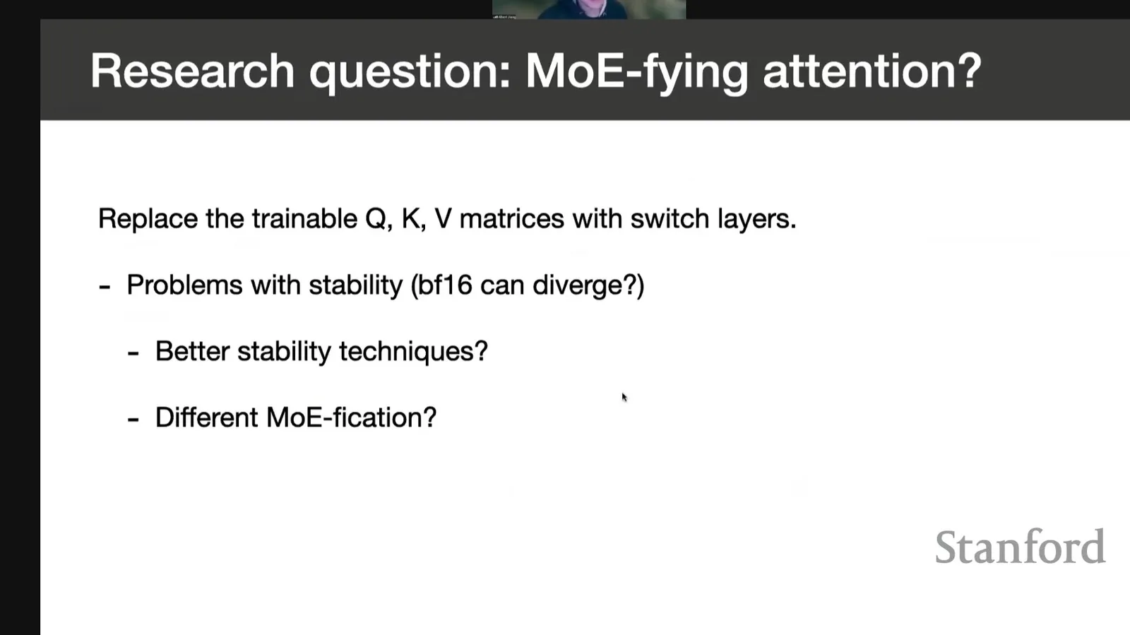
既然扩 MLP capacity 有效，自然问题是把 Q/K/V projection 也变成 switch layers。课程指出这条路线早已有实验，但数值稳定性是现实障碍：某些设置在 fp32 可训练，换到 bf16 会 diverge。由于现代大模型训练依赖低精度效率，能否稳定训练比纸面参数节省更关键。

\lecturefigure{slide-13-moe-attention-question.jpg}{开放问题：把 attention projection 也改成 MoE}{Stanford Online 官方录像 00:14:06}

背景概念：bf16 stability

bf16 保留与 fp32 相同数量级的 exponent bits，但 mantissa 更短，乘加、softmax、normalization 与 router logits 的舍入误差更明显。训练是否 diverge 取决于 scaling、normalization、optimizer、initialization 和 kernel implementation，不能只归因于“低精度不好”。

\teachervoice{00:12:38--00:14:03，Albert 把 MoE attention 留作明确 open research question：已有尝试在 bf16 下可能 diverge，未来需要更好的 normalization 或稳定化技术。}

本章小结

性能图支持一个有限结论：在相近 active parameters 下，Mixtral 的 capacity-to-compute tradeoff 很强，knowledge-heavy tasks 的增益尤其突出。它们不证明 MLP 独占知识，也不证明 active parameter 等于真实服务成本。MoE-fying attention 则提醒我们：结构扩展必须穿过低精度稳定性这一工程门槛。

四个 myths：从模型名字走向系统账本

课程中最具教学价值的部分，是连续拆解四个直觉错误。它们分别混淆 expert identity、total parameters、active compute 与 semantic specialization。本章逐个给出可计算的替代解释，并把 Q&A 中的 memory、communication 与 throughput 补进来。

Myth 1：Mixtral 只有八个全局 experts

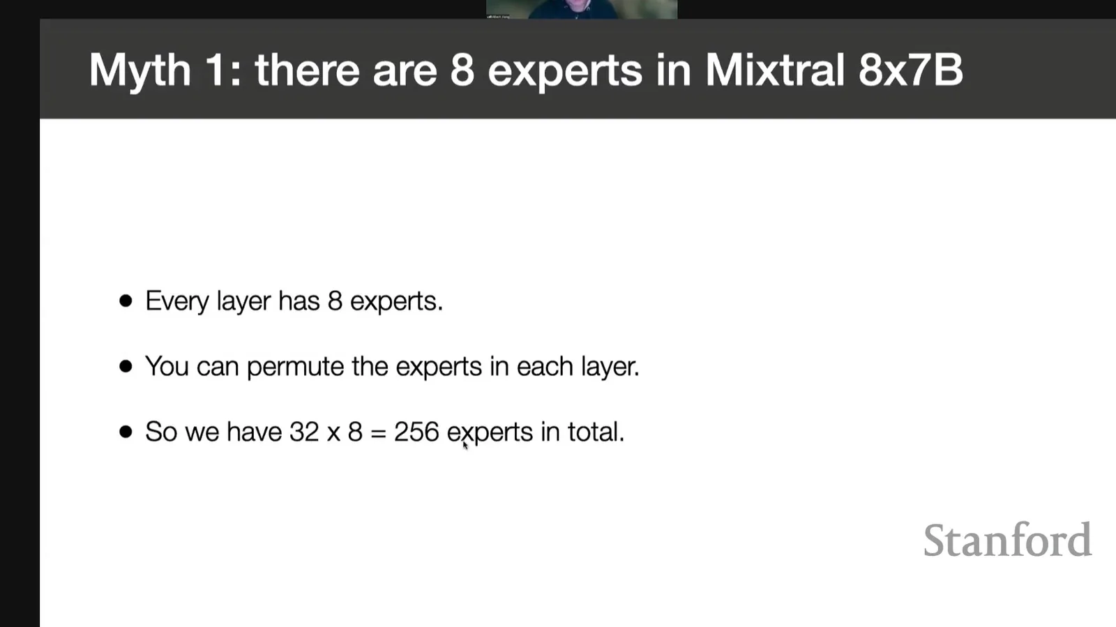
上一章已经说明 Mixtral 只在每层 MLP 路径引入稀疏 experts；这里首先纠正由“8x7B”命名诱发的全局角色想象。读下面的结构图时，应先区分“每层有几个可选 MLP”与“全模型有几个可跨层追踪的身份”，再判断 expert 编号能否承载语义。“8x7B”容易让人想象八个贯穿所有层的专家，实际却是每个 Transformer layer 都有八个 expert MLP；不同层的 expert 0 没有共享 identity。若有 \(N=32\) 层，结构上存在 \(32\times 8=256\) 个 layer-local expert modules。

\lecturefigure{slide-14-myth-eight-experts.jpg}{Myth 1：每层都有八个 experts，而非八个全局 experts}{Stanford Online 官方录像 00:15:12}

同一层内 expert label 具有 permutation symmetry。对任意 expert permutation \(\pi\)，若同时置换 expert weights 与 router output channel，函数保持不变：

\[ \sum_i g_i(x)E_i(x)=\sum_i g_{\pi(i)}'(x)E_{\pi(i)}'(x). \]

因此“expert 3”只在固定 checkpoint、固定 layer、固定 labeling 下有意义，不能跨层或跨训练 run 比较编号。

\teachervoice{00:14:15--00:15:09，Albert 说模型命名可能造成误解：每层八个专家，层内编号可置换；所以总共是许多 layer-local experts，而不是八个长期角色。}

不要跨层追踪 expert 编号

Layer 15 的 expert 3 与 layer 31 的 expert 3 没有天然语义连续性。若研究“同一个 expert 的成长”，必须先定义可比 alignment，而不是只比较数组下标。

\subsection{Myth 2：\texorpdfstring{\(8\times 7\mathrm{B}=56\mathrm{B}\)}{8 x 7B = 56B} 就是精确参数量}

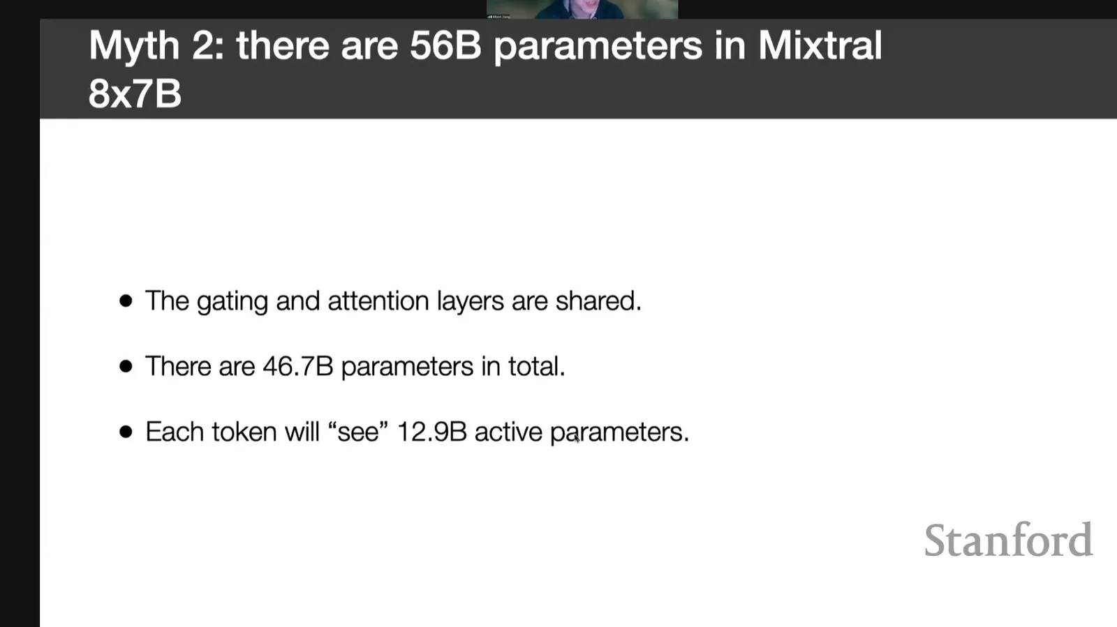
简单乘法忽略 shared embeddings、attention、normalization 和 router。课程给出约 46.7B total parameters 与 12.9B active parameters。真正需要记住的不是小数，而是 decomposition：总参数计算所有 expert weights，活跃参数只计算当前 token 选中的两个 experts，加上始终执行的 shared parts。

\lecturefigure{slide-15-myth-56b.jpg}{Myth 2：shared attention 使总参数不是简单的 56B}{Stanford Online 官方录像 00:15:37}

定义 expert fraction

\[ \rho=\frac{kP_e}{P_s+kP_e}, \]

它表示活跃路径中 expert MLP 占比。即使 \(k/E=1/4\)，整体 active/total ratio 也不严格是四分之一，因为 shared parameters 在分子分母都出现。

参数量报告的最小完整格式

至少同时报告：total parameters、active parameters per token、number of experts \(E\)、top-\(k\)、shared attention 配置和精度。只写“13B-class”会隐藏 46.7B 权重驻留；只写“47B model”又会隐藏每 token 稀疏执行。

\teachervoice{00:15:09--00:15:41，讲者纠正 56B 说法：attention 与 gating 共享，整体约 46.7B；每个 token 约看到 12.9B active parameters，而不是 14B。}

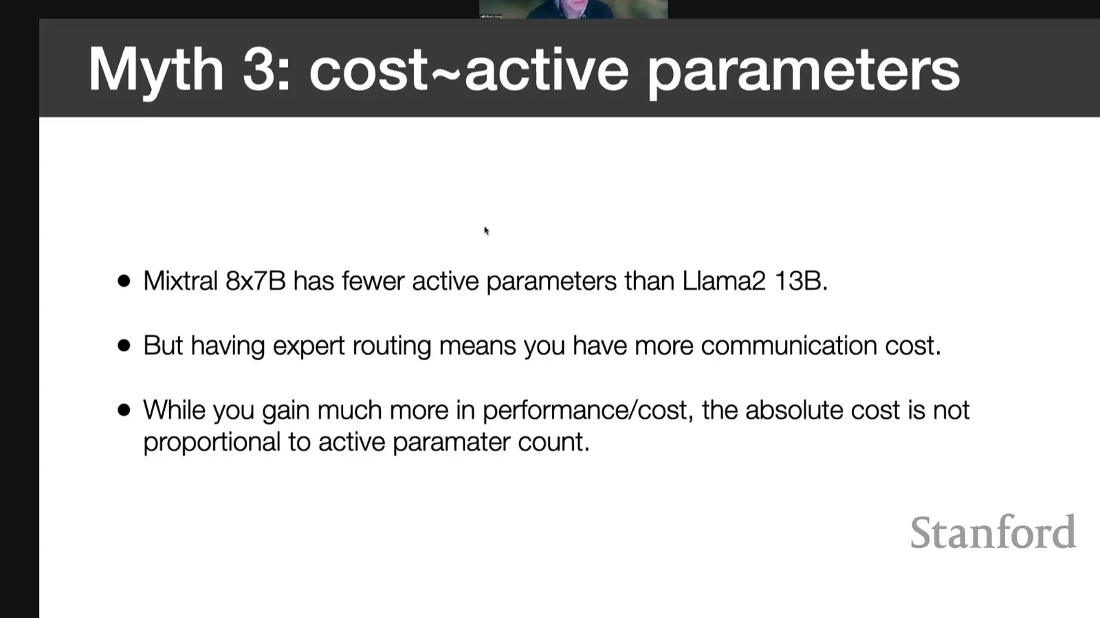
Myth 3：cost 与 active parameters 成正比

如果模型只在单卡上顺序执行，active parameters 是 FLOPs 的重要 proxy；一旦 experts sharding 到多卡，token 必须根据 router 决策重排并发送。Sharding（分片）指把不同 expert weights 放在不同 devices 上，使每卡不再复制全部 experts；它节省每卡存储，却引入 dispatch/combine communication。

\lecturefigure{slide-16-myth-cost-active.jpg}{Myth 3：active parameters 不能代表全部 serving cost}{Stanford Online 官方录像 00:16:42}

一个 batch 有 \(T\) 个 tokens，expert \(i\) 接收 \(n_i\) 个 token，则理想均匀负载为 \(T k/E\)。定义 imbalance ratio

\[ I=\frac{\max_i n_i}{Tk/E}. \]

\(I=1\) 表示最均匀；\(I>1\) 表示最忙 expert 超过平均。并行 step 往往由 \(\max_i n_i\) 决定，因此少数热点可让其他 devices 空等。

首次使用：expert parallel all-to-all

Expert parallelism 把 experts 分片到 ranks。Dispatch all-to-all 先把每个 token 发到目标 expert 所在 rank；expert 计算后，combine all-to-all 把输出送回原 rank。跨 node 通信通常比同 node GPU interconnect 更慢，所以 topology 与 placement 会改变 latency。

\teachervoice{00:15:41--00:16:49，Albert 明确反对把 cost 与 active parameter count 绑定。动态 routing 需要发送 token，无法预先固定路径，所以实际 serving 比同 active-size dense model 多出通信成本。}

Inference load balance：最慢 expert 决定这一轮何时结束

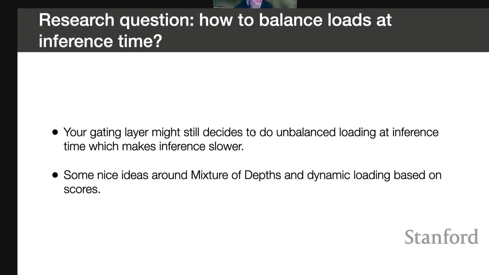
负载平衡不只是 training auxiliary loss。Inference 时真实 prompt distribution 可能让 router 偏向少数 experts，形成 straggler。即使平均计算量正确，只要某个 expert queue 过长，整个 batch 的 combine 阶段就必须等待它完成。

\lecturefigure{slide-17-inference-load-balance.jpg}{开放问题：怎样在 inference 时平衡 expert loads}{Stanford Online 官方录像 00:17:36}

常见 capacity 表达为

\[ C=\left\lceil \alpha\frac{Tk}{E}\right\rceil, \]

其中 \(\alpha\ge 1\) 是 capacity factor。若 expert 收到超过 \(C\) 的 token，可以 drop、reroute 或延迟处理；每种策略都会在 quality、latency 与 determinism 间交换。

训练均匀不保证线上均匀

Training data 的 router distribution 可能接近均匀，生产 prompt 仍可能集中在某些模式。线上应记录 per-expert token count、queue time、drop/reroute rate 和 tail latency，而不是只看平均 tokens/expert。

\teachervoice{00:16:49--00:17:36，讲者把 inference load balance 描述为等待最慢 expert 的问题，并提到 capacity-aware neighbor routing、mixture of depths 等探索。}

Compressing SMoEs：量化、offload 与 sparsification 不是一回事

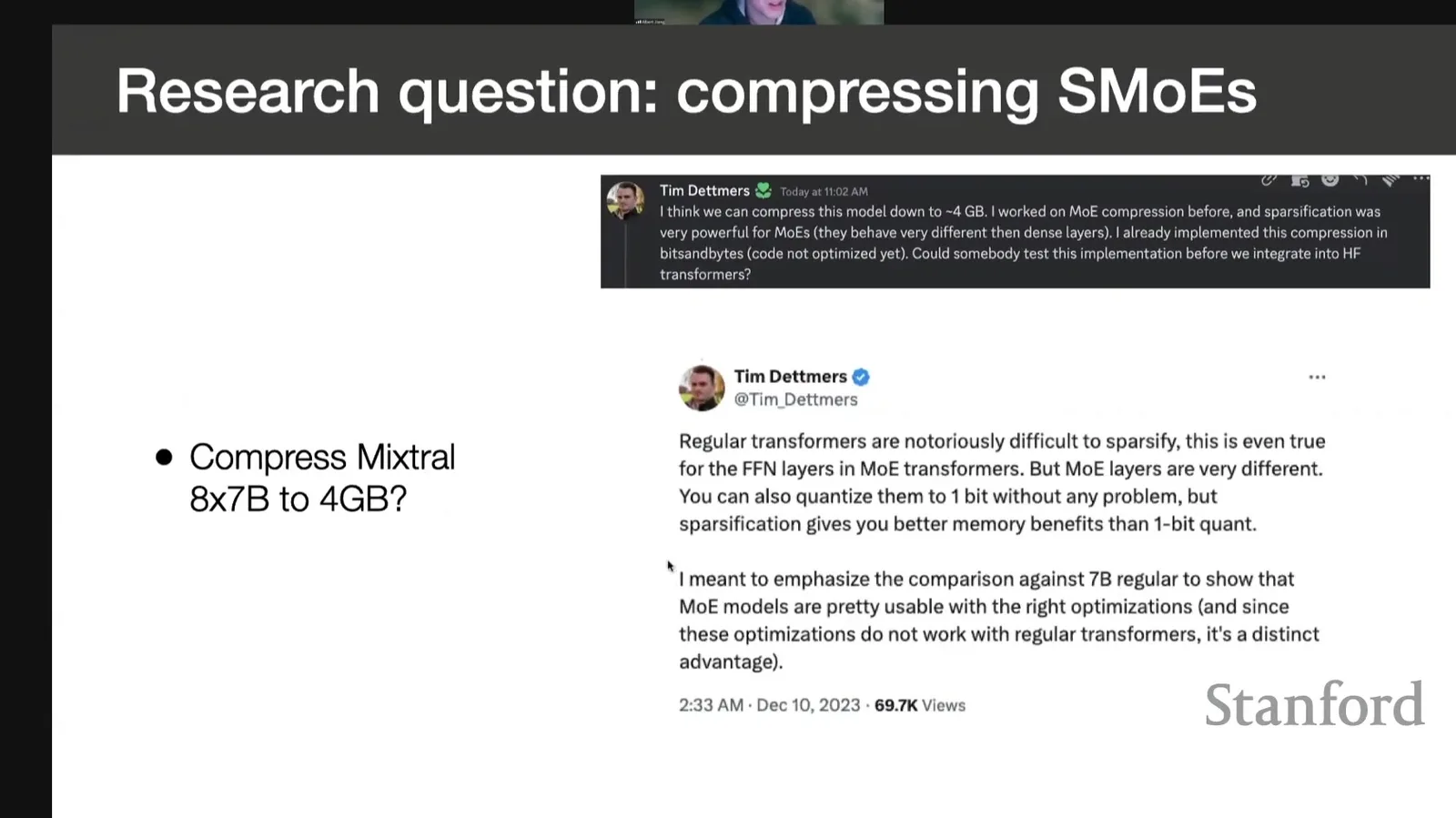
课程把压缩作为 open question，而不是已经完成的 recipe。Quantization（量化）降低每个 weight 的 bit 数；CPU offload 把部分 experts 从 GPU HBM 移到 CPU DRAM，需要时传输；sparsification 则尝试删除或置零 expert 内部不重要权重。这三者优化的资源不同，代价也不同。

\lecturefigure{slide-18-compressing-smoe.jpg}{开放问题：能否把 SMoE 压缩到极小内存}{Stanford Online 官方录像 00:19:07}

若 total parameters 为 \(P\)，每参数 \(b\) bit，理想权重存储下界为

\[ M_{\text{weights}}=\frac{Pb}{8}\ \text{bytes}. \]

实际还要加 scale/zero-point、KV cache、activation workspace、router buffers 和 framework metadata。Offload 则增加近似传输时间

\[ t_{\text{transfer}}\approx \frac{M_{\text{moved}}}{B_{\text{CPU--GPU}}}, \]

其中 \(B_{\text{CPU--GPU}}\) 是有效互连带宽。

术语消化：三类压缩

方法	主要节省	主要风险
Quantization	每个 weight 的 bytes	精度损失、dequant kernel、scale overhead
Offload	GPU resident memory	PCIe/NVLink transfer、cache miss、tail latency
Sparsification	有效 nonzero weights/FLOPs	不规则 kernel、质量退化、重新训练

\teachervoice{00:17:36--00:19:15，Albert 引用社区对极端压缩的乐观猜测，但承认截至讲课时还没有看到令人信服的 extreme SMoE sparsification 结果；这是一条研究议程，不是发布承诺。}

本章小结

四个 myth 的共同根源，是把名称当成系统模型。正确替代是：experts 是 layer-local 且可置换；total 与 active parameters 必须分开；serving cost 还包含 communication 与 imbalance；semantic domain specialization 既非必要也未被 routing 图证明。Load balance 与 compression 则把这些概念落到真实硬件约束。

Routing interpretation：离散 gate 提供证据，但不自动给出语义

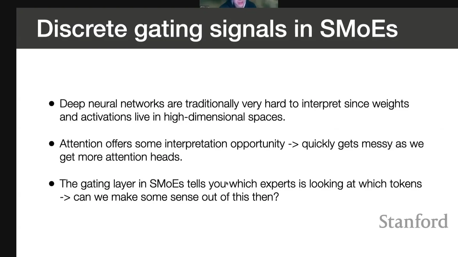
Dense network 的 activation 位于高维连续空间，很难直接解释；SMoE router 至少给出离散 expert IDs 和 gating weights，让研究者可以统计 token 到 expert 的分配。本章沿课程的三个分析层次展开：domain histogram、consecutive-token persistence、token-level map；最后再讨论社区 expert ablation 和“expert 不是 domain”的结论。

为什么 discrete gate 看起来更可解释

Router 每层为 token 产生一个小集合 \(S_k(x)\)，这比数千维 activation 更容易计数。研究者可以问：不同数据 domain 是否偏向不同 experts？相邻 token 是否保持同一路由？删除某个 expert 会怎样？但这些问题只产生 observable correlations，解释仍需要对照实验。

\lecturefigure{slide-19-discrete-gating.jpg}{Discrete gating signals 为 SMoE interpretation 提供新观测量}{Stanford Online 官方录像 00:20:19}

对 domain \(d\)、layer \(\ell\)、expert \(i\)，routing frequency 可写成

\[ p_{\ell}(i\mid d)=\frac{\#\{x\in d:i\in S_k^{(\ell)}(x)\}}{k\,|d|}. \]

若完全均匀，\(p_{\ell}(i\mid d)\approx 1/E\)。偏离均匀只是“该 domain 的 token 更常选这个 expert”，不是“这个 expert 的语义就是该 domain”。

Attention weight 与 router ID 都不是因果解释

可视化告诉我们模型看了什么或选了谁，但不等于该组件对输出具有唯一因果作用。需要 intervention、ablation、counterfactual routing 或 retraining 才能更接近因果结论。

\teachervoice{00:19:15--00:20:24，讲者认为 discrete gate 比 dense activation 提供了“incredible opportunity”，但他的提问仍是“can we make some sense out of this”，而非宣布可解释性已经解决。}

Domain histogram：中层 spike 有趣，但证据仍弱

实验把 The Pile 的不同 validation subsets 输入模型，统计 layer 0、15、31 的 expert selection。浅层与深层大体接近均匀，中层某个 expert 对 DeepMind Mathematics/GitHub 有较高选择率。读图时先看 \(1/E=12.5\%\) baseline，再比较层间变化，而不是给颜色直接命名。

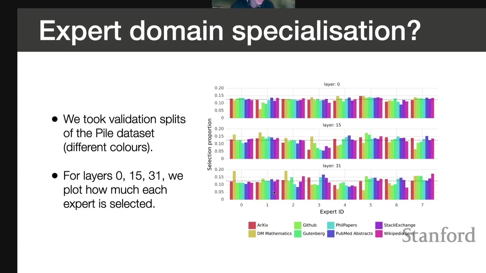
\lecturefigure{slide-20-domain-specialisation.jpg}{The Pile 不同 domains 在浅层、中层和深层的 expert routing 分布}{Stanford Online 官方录像 00:22:39}

读图：三层分别可能看见什么

Layer 0 接近 raw token，路由可能受字符、标点和局部句法影响；中层包含更多组合表示，因此出现 domain-correlated spike；最后一层接近 decoding objective，分布又可能趋于共享输出需求。这个叙述是可检验 hypothesis，不是由一张图唯一确定。

\teachervoice{00:20:24--00:22:28，Albert 说 layer 15 expert 3 的 math/code spike “interesting”，随后马上补充 highly speculative、cannot conclude much。这个自我限制必须保留。}

Consecutive tokens：routing persistence 在中层更强

Domain histogram 只告诉我们不同数据子集的总体选择比例，无法判断 router 是否在一个局部片段内保持决策。第二个实验因此把问题从“什么 domain 更常选谁”改成“相邻 token 是否连续选择同一 expert”。读图时先确认 top-1 与 top-2 两种事件的随机 baseline，再比较浅层、中层和深层，而不要把连续性直接解释为主题专门化。若 top-1 在八个 experts 间独立均匀，随机 baseline 为 \(1/8=12.5\%\)；若比较“下一 token 是否把该 expert 放在 top-2”，baseline 会更高。图中 layer 15 的 persistence 明显高于随机，layer 0 较弱，layer 31 又回落。

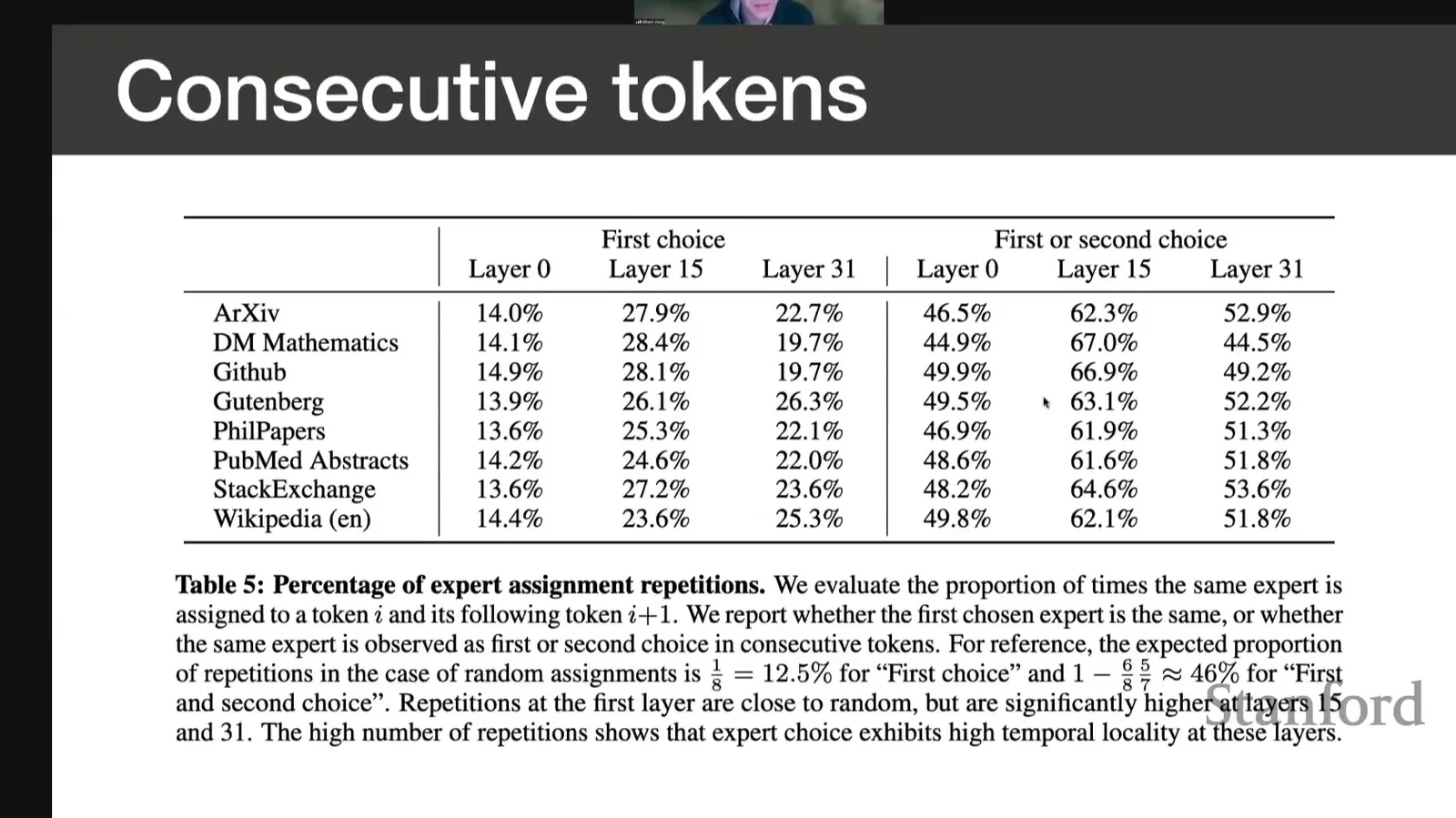
\lecturefigure{slide-21-consecutive-tokens.jpg}{相邻 token 继续选择同一 expert 的频率}{Stanford Online 官方录像 00:25:13}

定义 top-1 persistence

\[ P_{\ell}^{(1)}=\Pr\!\left(e_{t+1}^{(1)}=e_t^{(1)}\right), \]

以及 set persistence

\[ P_{\ell}^{(2)}=\Pr\!\left(e_t^{(1)}\in S_2(x_{t+1})\right). \]

它们衡量局部路由连续性，却不能说明连续 token 共享“主题专家”；subword、syntax、position 或 hidden-state smoothness 都可能造成 persistence。

\teachervoice{00:22:46--00:25:18，讲者逐层解释 random baseline 与 observed frequency：layer 15 约为最强，最后一层仍高于随机但有所回落，并明确说需要更细分析。}

Token map：颜色看起来有模式，语义却不整齐

第三个实验把代码、算术和选择题 token 按 expert 着色。某些数字或局部片段出现相似颜色，但整体没有“代码全部进 expert A、数学全部进 expert B”的清晰划分。图像最重要的教学作用，是让读者亲眼看到 expert routing 的碎片化，而不是制造一个漂亮 taxonomy。

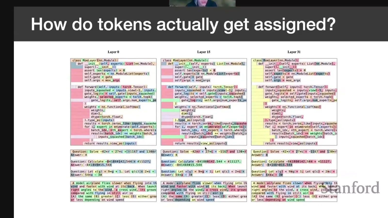
\lecturefigure{slide-22-token-assignment.jpg}{代码、算术与问答样本的 token-level expert assignment}{Stanford Online 官方录像 00:26:13}

读图：先看局部连续，再看跨样本一致性

第一步找同一序列中的连续颜色块；第二步比较同类 token 在不同样本是否保持颜色；第三步跨 layer 比较。只有多样本、跨层、跨随机种子都稳定，才值得尝试给 expert 语义命名。

\teachervoice{00:25:18--00:26:19，Albert 观察到一些 digits 被送到同一 expert，但总体“doesn't seem to be much specialization”。课程没有从 token map 推出明确 domain taxonomy。}

Myth 4：为什么纯 domain experts 还可能降低利用率

假设只有两个 experts 专门处理 code，那么长代码序列会把大量 token 压到这两个 experts，其余六个空闲；这既产生 load imbalance，也浪费并行 capacity。更合理的 specialization 可能是跨 domain 共享的 latent features，使所有 experts 在不同输入上都能被利用。

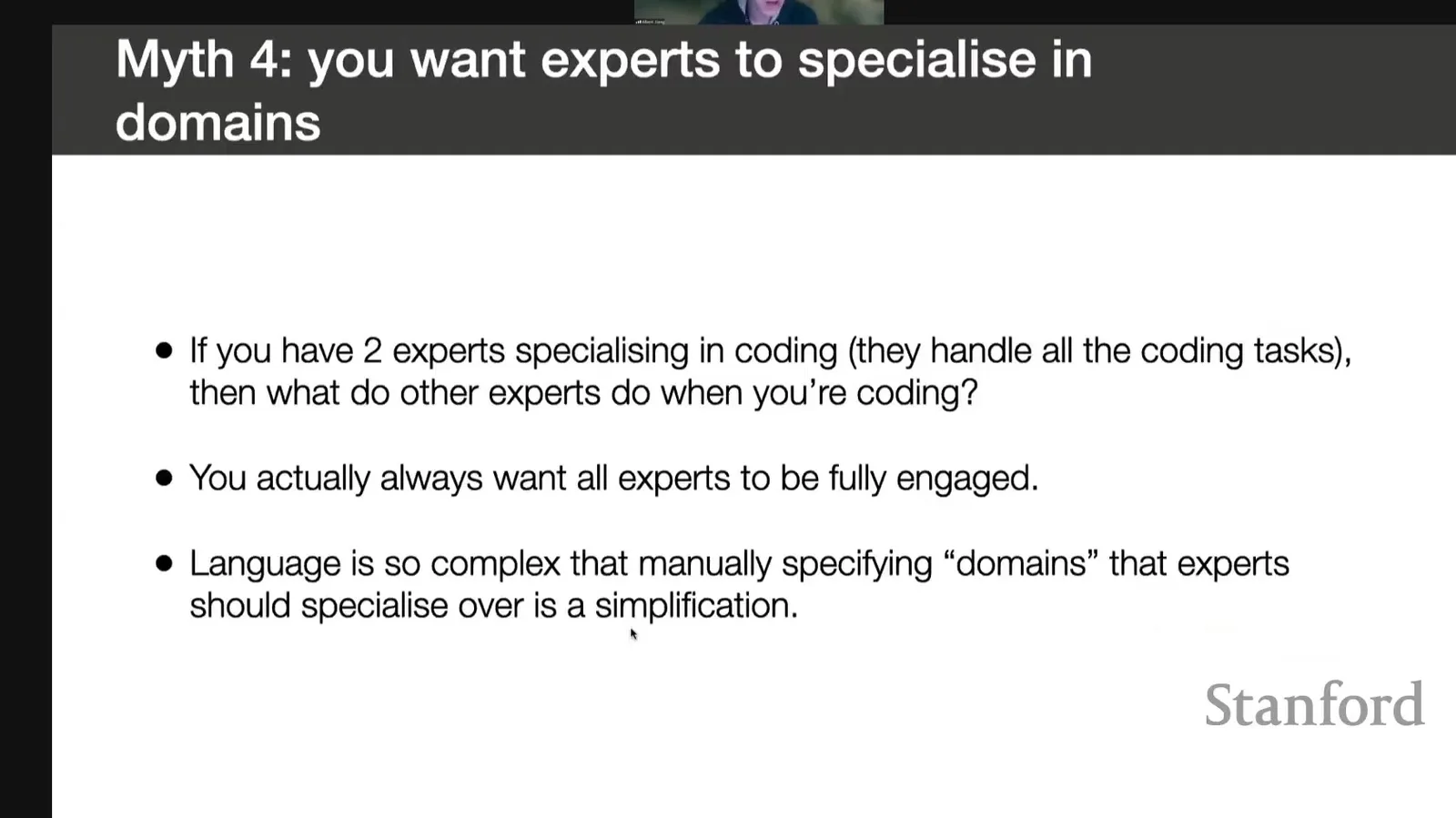
\lecturefigure{slide-23-myth-domain-specialisation.jpg}{Myth 4：最优 experts 不一定按人类 domains 分工}{Stanford Online 官方录像 00:27:15}

若 domain \(d\) 的 token 全部路由到子集 \(A_d\)，利用率上界近似为

\[ U_d=\frac{|A_d|}{E}. \]

例如 \(|A_d|=2,E=8\) 时，单一 domain batch 最多充分使用四分之一 experts。现实 router 可 top-two 混合并跨 feature 分工，但公式揭示“干净 domain 专家”与高利用率之间的张力。

Specialization 的更稳妥定义

不要先指定 expert 名称，再找例子；应测量路由分布、representation probe、causal ablation 与 load behavior，再描述某个 expert 对哪些 features 敏感。Feature 可以跨代码、数学和自然语言同时出现。

\teachervoice{00:26:20--00:27:22，讲者用 coding experts 的反例说明：若代码 token 只进两个 experts，其他 experts 就站着不工作；语言太复杂，不应把 specialization 简化成高层 domains。}

Treasure hunt：开放权重让社区快速做 intervention

模型发布约一天后，社区尝试移除特定 expert，发现删除某一编号会让 MMLU 大幅崩溃，并做成“一个人在干活、其他人在围观”的 meme。这个结果很醒目，但它可能反映 router calibration、layer-specific bottleneck、implementation 或 distributed ablation 方法；不能直接证明一个 expert 存了全部知识。

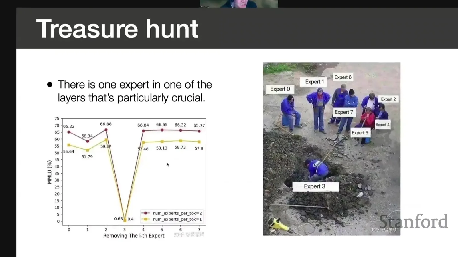
\lecturefigure{slide-24-treasure-hunt.jpg}{社区 expert ablation、MMLU 崩溃与开源 meme}{Stanford Online 官方录像 00:28:31}

定义删除 expert \(i\) 后的 metric change

\[ \Delta_i=m(\theta_{-i})-m(\theta), \]

其中 \(\theta_{-i}\) 表示禁用某 expert 的干预模型。大的负 \(\Delta_i\) 证明该干预影响输出，却不能区分 expert 本身知识、router re-normalization 或 downstream distribution shift。

Ablation 设计必须记录四件事

删除的是一个 layer 的 expert 还是所有层同编号？Gates 是否重新归一化？Overflow token 如何处理？Metric 是否对输出格式敏感？不记录这些，社区结果只能是线索。

\teachervoice{00:27:22--00:28:38，Albert 把这个 24 小时内出现的社区发现当作“why we love open source”的例子；价值在于快速 intervention，不在于 meme 已经解释模型。}

最终解释议程：寻找 latent feature subspaces

课程最后没有给 experts 贴标签，而是提出更难的问题：experts 可能编码人类概念的线性组合，或对某个 feature subspace 敏感。未来研究需要把 routing stats 与 representation analysis、causal patching、expert swapping 和 controlled retraining 结合起来。

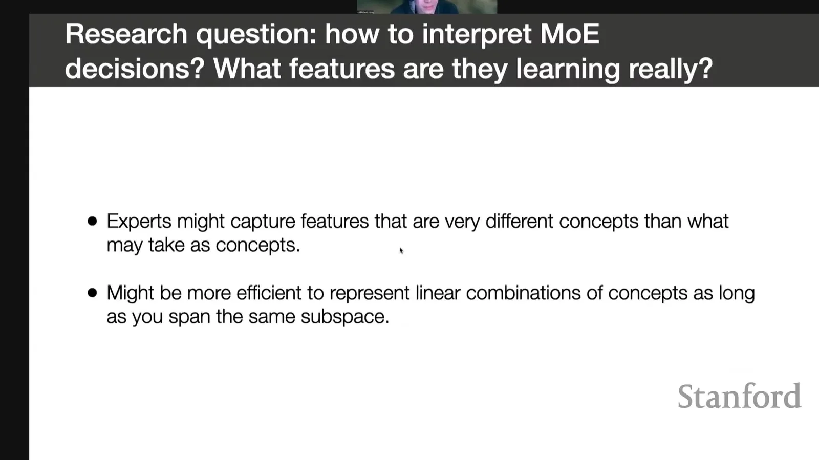
\lecturefigure{slide-25-interpret-moe-decisions.jpg}{开放问题：experts 真正学习了哪些 features}{Stanford Online 官方录像 00:29:11}

从可视化到解释的证据阶梯

Routing histogram \(\rightarrow\) token map \(\rightarrow\) controlled ablation \(\rightarrow\) counterfactual rerouting \(\rightarrow\) retraining/feature recovery。越往后越接近因果，但成本也越高。单张 histogram 只能位于阶梯起点。

\teachervoice{00:28:38--00:29:30，讲者认为 experts 可能捕获与人类概念不同的 features，甚至是多个概念的线性组合；真正问题是怎样恢复其 subspace。}

本章小结

Discrete routing 确实给 interpretability 增加了可观测变量：domain frequency、routing persistence、token assignment 和 ablation sensitivity。但所有结果都指向同一谨慎结论：experts 具有结构化行为，却未按简单人类 domain 分工。最有价值的研究方向是把离散 gate 与因果干预、representation geometry 和系统负载联合起来。

Q&A 工程综合：什么时候 MoE 值得，什么时候 dense 更诚实

主讲结束后的 Q&A 占整段录像一半以上，且补上 slides 没有展开的部署条件。本章不按提问顺序堆答案，而按系统因果重组：edge/cloud memory、expert parallel communication、batch throughput、domain adaptation、RAG、modular experts、gradient flow 与 larger expert counts。

Edge versus cloud：稀疏执行不等于稀疏驻留

对 memory-constrained edge device，dense model 往往更直接，因为 MoE 仍需存所有 experts。若权重全驻 GPU，resident memory 近似 total parameters；若只驻 CPU，GPU 虽省内存，却需要频繁搬运。Centralized serving 拥有多卡、高带宽和大 batch，才更容易把稀疏执行转成吞吐收益。

Edge 选型的第一问

先问设备能否容纳 total weights，而不是只问 active parameters。一个 12.9B-active 的 MoE 仍可能需要约 46.7B 参数的存储。若单机只能容纳 7B dense，不能因为 top-two 就假设 Mixtral 也等价占用 13B。

\teachervoice{00:31:45--00:33:10，Albert 纠正现场提问者：edge 上 dense model 可能更合适，因为 sparse inference 仍要加载所有 experts；MoE 的 cost/performance 优势更适合集中式 serving。}

Batch size 与 throughput：为什么高流量更可能摊薄复杂度

在小 batch 下，不同 experts 收到的 token 少且不均，all-to-all 与 kernel launch 难以摊薄；高 batch 可把更多 token 聚合成较大的 expert GEMM，提高 arithmetic intensity。可用简化吞吐模型表示

\[ \operatorname{throughput}\approx \frac{T}{\max_i t_{\text{expert},i}+t_{\text{dispatch}}+t_{\text{combine}}}. \]

提高 \(T\) 只有在 expert batches 变大且 imbalance 可控时才有帮助；若热点 expert 同比例变热，tail 仍由它决定。

读系统指标：平均 latency 不够

同时报告 tokens/s、time-to-first-token、inter-token latency、P50/P95/P99、per-expert batch size、all-to-all bytes 和 HBM occupancy。MoE 可能提高 aggregate throughput，却让单请求 latency 或 tail 更差。

\teachervoice{00:42:47--00:43:33 与 00:54:56--00:56:17，讲者两次强调 use case：高 batch、high-volume serving 更能体现 MoE throughput；小规模和显存受限环境则承担更多复杂度。}

Communication topology：跨 node 比跨 GPU 更贵

Expert parallelism 的成本不仅由 bytes 决定，还由 topology 决定。同 node GPU 可能通过 NVLink/NVSwitch 通信，跨 node 则经过 InfiniBand/Ethernet 与 network stack。若一个 expert 本身跨多卡做 tensor parallel，token dispatch 与 expert 内 collectives 还会叠加。

专家数越多不一定越快

增加 \(E\) 可以提供更多 routing choices，却会让每个 expert 的 batch 变小、placement 更碎、metadata 与 communication 更复杂。若 experts 跨 nodes，网络延迟可能吞掉稀疏计算收益。

\teachervoice{00:40:43--00:41:36，Albert 指出 GPU-to-GPU 已经昂贵，node-to-node 更昂贵；通信成本与 token routing 及硬件放置相关，如何继续扩展仍是开放问题。}

Memory、offload 与 dense-equivalent heuristic

Q&A 给出三个容易混淆的判断。第一，naive resident memory 接近 46.7B/7B 的权重比例；第二，CPU offload 可省 GPU HBM，却增加参数搬运；第三，用 \(\sqrt{P_{\text{active}}P_{\text{total}}}\) 估计 dense-equivalent capability 只能是粗略 rule of thumb。

几何平均 heuristic 为

\[ P_{\text{equiv}}\approx \sqrt{P_{\text{active}}P_{\text{total}}}, \]

但能力还受 training tokens、data quality、optimizer、router balance 和 architecture 影响。它不能替代同训练预算的 controlled scaling experiment。

\teachervoice{00:50:42--00:52:42，讲者说全驻显存时 memory 更接近 total parameter ratio；CPU offload 会损失传输效率；几何平均可作 rule of thumb，但前提是训练 token 与质量等条件相当。}

Knowledge versus reasoning：benchmark category 不是机制探针

听众问 Mixtral 为什么 reasoning 更好，Albert 的回答很克制：数学 benchmark 中，模型可能真正推理，也可能记住可调用 lemma 或模式；knowledge 与 reasoning 的边界本就模糊。因此更高分不证明 MoE 学到新内部算法，更不证明 attention/MLP 已被功能拆开。

能力标签不能代替过程证据

若要研究 reasoning mechanism，应加入 out-of-distribution composition、intermediate trace、counterfactual perturbation 和 memorization control。仅靠 benchmark 名字中的 “reasoning” 无法判定计算过程。

\teachervoice{00:53:26--00:54:41，讲者认为 Mixtral 的 knowledge 增益明确，但 knowledge 是否诱发 reasoning 改进高度 speculative；benchmark 自己也难区分 recall 与 reasoning。}

Domain adaptation、RAG 与 modular experts 是三条独立轴

MoE 增加 model capacity，continued pretraining/fine-tuning 改变 domain distribution，RAG 在 inference 时检索外部证据。三者可以组合，不能互相替代。一个 medical dense model 通过专门数据训练后，可能比通用 MoE 更强；一个 MoE 也可以接 RAG；把新 medical expert 插入 checkpoint，则还需训练 router 学会何时使用它。

三条轴的区别

机制	改变什么	不自动解决什么
MoE	参数容量与 token execution path	外部知识更新、明确 domain label
Domain tuning	权重对目标数据分布的适配	实时事实、检索 provenance
RAG	inference-time context/evidence	模型内部参数容量与 routing balance

\teachervoice{00:43:50--00:44:40，Albert 说专门 domain pretraining/fine-tuning 很难被通用模型击败，而且 Mixtral experts 并非显式 medical/coding experts。00:59:02--00:59:43，他又说明 RAG 与 dense/MoE 是正交组合。}

Expert swapping：可行不等于 plug-and-play

若替换某个 expert，router 原 logits 与新 expert behavior 不匹配。即使 tensor shape 一致，模型也不知道何时把 medical token 路由到新模块；还可能破坏 residual statistics。最低限度需要 router/新 expert adaptation，并检查其他 experts 的负载与能力退化。

替换 expert 后的最小验证流程

load_base_moe_checkpoint()
replace_one_expert_with_domain_module()
freeze_or_partially_train_shared_attention()
train_router_and_new_expert_on_mixed_data()
measure_load_balance_and_general_capability()
run_domain_eval_and_out_of_domain_regression()

\teachervoice{00:59:43--01:00:54，讲者认为 expert swapping 有研究潜力，但明确要求继续训练 gating layers，让 router 学会新的 domain expert 应在何时被调用。}

Gradient flow 与 training cost：-\(k\)top-k 仍可端到端优化

Q&A 最后纠正另一个误解：router 虽然产生离散 top-\(k\) selection，选中路径上的 gating 与 expert operations 仍可微，模型可端到端训练。严格来说 top-\(k\) 边界是分段/非光滑的，但实际优化对当前选中 experts 传播梯度，并配合 load-balancing objectives。

训练成本可概括为

\[ C_{\text{train}}\approx C_{\text{active forward/backward}}+C_{\text{router}}+C_{\text{communication}}+C_{\text{balance}}. \]

它通常更接近同 active-size dense model，而不是 total-size dense model，但 extra communication 与 optimizer/state storage 仍存在。

Optimizer state 仍按训练参数计费

Adam/AdamW 为每个可训练参数维护一阶矩 \(m\) 与二阶矩 \(v\)，再加 parameter 和 gradient。若所有 expert weights 都训练，optimizer state 与 total trainable parameters 相关，而不是只与当前 token active path 相关；分布式训练常需 state sharding 来降低每卡内存。

\teachervoice{01:01:10--01:02:08，Albert 说 routing path 可端到端 differentiable，训练计算大致像 13B active model，但还要承担额外 communication。}

更多 experts：选择空间增加，服务难度也增加

把 expert 数提高到 64/128，可以给 router 更细的选择空间，也可能让 experts 更专门化；但每个 expert batch 更小、placement 跨更多 nodes、all-to-all 更复杂，甚至单个 expert 都可能无法放进一张 GPU。模型提供商可通过专门基础设施隐藏复杂度，自部署用户则必须面对它。

扩大 \(E\) 前的四个问题

每个 expert 是否足够大以学习有用 features？每 step 每 expert 有多少 token？Experts 是否跨 node？Serving volume 是否足以形成大 GEMM？若这些问题没有正面答案，更多 experts 可能只增加 orchestration cost。

\teachervoice{01:02:26--01:04:14，讲者认为更多 experts 很有研究吸引力，却会让 multi-node serving 和 communication 更难；对单 GPU，他更倾向 dense 或 heavily quantized MoE，并判断量化后的 Mixtral 8x7B 仍可实践。}

本章小结

Q&A 把 slides 的算法叙述变成部署条件：MoE 更适合有足够 resident memory、interconnect 与 serving volume 的环境；edge 与小 batch 未必划算。Domain tuning、RAG 和 MoE 彼此正交；expert swapping 需要 router adaptation；训练 compute 接近 active path，但 optimizer state、communication 与 load balancing 仍按更完整系统计费。

结论：稀疏容量的收益来自选择，代价也来自选择

主讲结论可以压缩为三个判断。第一，SMoE 用稀疏 activation 换取更大知识容量，并能处在优秀的 active-compute frontier；第二，训练和 serving 能做到高效，但绝不只由 active parameter count 决定；第三，expert specialization 有结构，却不像“代码专家/数学专家”那样直接。最后一张 slide 把 architecture 与 interpretability research 同时保留为开放方向。

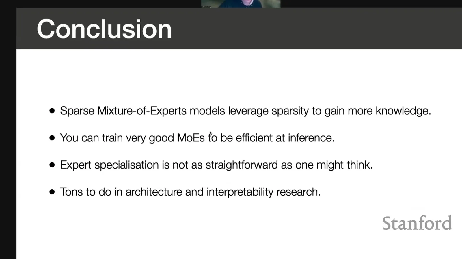
\lecturefigure{slide-26-conclusion.jpg}{Albert Jiang 对 Sparse MoE、效率与 expert specialization 的总结}{Stanford Online 官方录像 00:29:38}

本讲最终公式：三本账必须一起报告

\[ \boxed{\text{Model decision}=f(P_{\text{total}},P_{\text{active}},M_{\text{resident}},C_{\text{comm}},I_{\text{load}},Q_{\text{quality}})} \]

其中 total/active 描述结构，resident memory/communication/load 描述系统，quality 描述任务证据。任何只保留一个变量的比较都可能误导。

\teachervoice{00:29:18--00:29:47，讲者的原始总结是：SMoE 借 sparsity 获得更多 knowledge，可以训练成高效 inference model，但 expert specialization 没有直觉上那么简单，architecture 与 interpretability 仍有大量工作。}

本章小结

Mixtral 的价值不在“八个专家”这个标签，而在 token-level conditional computation：总容量增长、活跃路径受控、router 动态选择。它同时创造了新的系统瓶颈和新的可解释观测量。只有把结构、硬件和证据放在一起，才能判断某个 MoE 是否真的优于 dense baseline。

总结与延伸

这堂课最值得迁移到其他模型的，不是一组 Mixtral 数字，而是一套审计方法：先确认 dense baseline，再写清 routing algorithm；同时报告 total/active/resident；把 communication 与 load balance 纳入成本；最后用 routing statistics 与 intervention 检查“experts”是否真的有可解释分工。

十五条核心结论

以下结论按结构、系统和解释三层组织，避免把模型名当作答案。

1. Mixtral 保留 Mistral 7B attention，只把每层 MLP 换成 top-two-of-eight experts。
2. GQA 减少 KV heads 与 KV cache；SWA 限制单层 attention neighborhood。
3. Router 为每个 token 独立打分、选 top-\(k\)、归一化并加权组合 expert outputs。
4. 每层都有八个 experts；expert 编号在层内可置换，跨层没有天然身份。
5. Total parameters、active parameters 与 resident memory 是三种不同量。
6. Active parameters 主要近似 per-token compute，不代表完整 latency 或 dollar cost。
7. Expert parallelism 需要 token all-to-all，跨 node topology 可能成为瓶颈。
8. Load imbalance 让最忙 expert 决定并行 step 的 tail。
9. 高 batch/高流量更容易把 expert GEMM 做大并摊薄 dispatch overhead。
10. MLP-knowledge hypothesis 有实验启发性，但不是功能定位定理。
11. 2024 benchmark 显示 knowledge-heavy gains 最大，却不能证明新 reasoning algorithm。
12. Discrete routing 提供可统计信号，但 routing frequency 不是语义或因果解释。
13. Clean domain experts 可能导致其他 experts 空闲，降低利用率。
14. Expert ablation 是重要 intervention，但必须记录 layer、gate normalization 与 overflow 处理。
15. MoE、domain tuning 与 RAG 是可组合的不同轴，expert swapping 还需要 router adaptation。

一张表串起结构、训练与 serving

为了把概念变成工程检查，下表给出每个阶段最应该观察的变量和常见误判。

阶段	关键观测量	常见误判
Architecture	\(E,k\)、shared/expert params、GQA/SWA	用模型名估参数量
Training	tokens/expert、aux loss、gradient、optimizer state	只按 active params 算内存
Placement	expert sharding、node topology、HBM	假设未激活 expert 不需驻留
Serving	batch、all-to-all、imbalance、tail latency	用 FLOPs 代替真实 cost
Interpretation	routing stats、ablation、counterfactual	给 expert 直接贴 domain 标签
Evaluation	task setup、active/total axes、history date	把 2024 plot 当当前排名

MoE 从架构到解释的最小审计框架。

实践用 MoE release checklist

下面的 checklist 用于审阅论文、模型卡或内部 release，重点是避免只展示 parameter headline。

Sparse MoE release checklist

report_total_and_active_parameters()
report_expert_count_topk_and_shared_modules()
report_weight_precision_and_resident_memory()
report_tokens_per_expert_and_load_imbalance()
report_expert_parallel_topology_and_all_to_all_cost()
compare_against_dense_models_at_compute_and_memory_budgets()
publish_routing_analysis_with_causal_controls()
document_quantization_offload_and_failure_cases()

看到 “13B active” 时立即追问

Checkpoint 总参数是多少？所有 experts 放在哪里？是单卡、单 node 还是跨 node？Batch size 多大？P99 latency 如何？是否发生 token drop/reroute？没有这些信息，active parameter headline 只描述局部计算路径。

自测问题

这些问题用于检查是否真正掌握三本账和 routing evidence。

1. 为什么 Mixtral 不是八个独立 7B 模型的 ensemble？
2. GQA 与 SWA 分别降低什么资源？
3. 写出 top-two routing 从 logits 到 weighted sum 的过程。
4. 为什么 \(8\times 7\mathrm{B}\) 不是 total 或 active parameter 的精确值？
5. Active parameters 为什么不能直接预测 serving latency？
6. Expert parallel all-to-all 在 dispatch 与 combine 两阶段分别做什么？
7. 为什么最慢 expert 会控制一个 batch 的完成时间？
8. Quantization、offload 与 sparsification 有什么区别？
9. Domain routing histogram 能证明什么，又不能证明什么？
10. 为什么纯代码 experts 可能降低整体利用率？
11. Expert ablation 需要记录哪些控制变量？
12. 为什么 RAG 与 MoE 不是替代关系？
13. 替换一个 expert 后为什么还要训练 router？
14. 更多 experts 在什么条件下可能反而降低 throughput？

拓展阅读

• Jiang et al., Mixtral of Experts：模型结构、性能与 routing analysis 的主论文。
• Jiang et al., Mistral 7B：GQA、SWA 与 dense baseline。
• Shazeer et al., Outrageously Large Neural Networks：sparsely-gated MoE layer。
• Fedus et al., Switch Transformers：大规模稀疏训练与 parallelism。
• 阅读这些论文时，同时记录 total/active parameters、precision、hardware、batch 与 communication；不要只摘 benchmark headline。