CS336 2026 Lecture 5:GPUs、Roofline 与 FlashAttention
本讲的问题:GPU 为什么既快又难用?
Lecture 5 把 Lecture 2 的 resource accounting 落到硬件:为什么 GPU 能支撑 scaling?为什么同样是 FLOPs,有的操作飞快,有的操作很慢?为什么 FlashAttention 这种算法能改变 attention 的实际速度?本讲的核心问题因此不是峰值 FLOP/s,而是算子能否把足够多的数据复用和并行工作送到执行单元,同时避免 HBM、调度与对齐成为瓶颈。
术语消化:GPU memory hierarchy
HBM 是 High Bandwidth Memory,GPU 上的大容量高带宽显存,容量大但离计算单元远;SRAM 是 Static Random-Access Memory,常对应片上 shared memory/cache,容量小但速度快;register 是每个 thread 私有的最快存储。GPU 优化的核心之一,就是让数据从 HBM 读进来以后尽量在 SRAM/register 附近复用,而不是频繁写回 HBM。
本讲主线
GPU performance 的核心不是“GPU 很快”四个字,而是让数据移动、并行执行和矩阵硬件匹配。低精度、fusion、recomputation、coalescing、tiling、FlashAttention 都是在减少 HBM 往返或提高数据复用。
GPU 为什么适合大规模深度学习
本节从 compute scaling 的历史讲到 GPU 与 CPU 的区别,再拆 SM、SP、warp、block、register、shared memory 和 HBM。
术语消化:SM、SP、warp、block
SM 是 Streaming Multiprocessor,是 GPU 上执行 thread blocks 的主要单元;SP/CUDA core 是 SM 内的标量执行单元;warp 是一组通常 32 个 lockstep 执行的 threads;thread block 是被调度到一个 SM 上的线程组。HBM 是 GPU 的高带宽显存,容量大但离计算单元远;SRAM/shared memory/register 更靠近 SM,容量小但快。
展开说明:GPUS
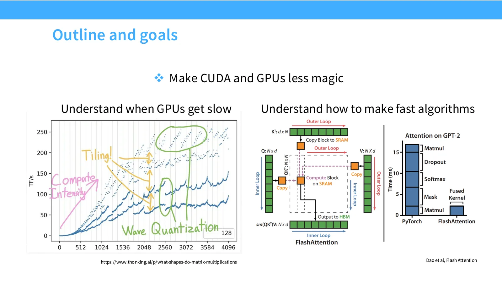
课程先用一张目标页明确方法:一端是“理解 GPU 何时变慢”,另一端是“把这些原因转化成快速算法”。因此本讲不会停留在 CUDA 名词解释,而会用 matrix shape、roofline、memory hierarchy 和 FlashAttention 把硬件现象与算法设计连起来。读后续性能图时,要不断问:这是峰值算力限制、带宽限制、并行度不足,还是 shape/alignment 让硬件单元闲置?
来源:CS336 Spring 2026 Lecture 5 官方幻灯片。
读图:两端目标必须同时验收
只理解 GPU block/warp 并不能自动写出高性能 kernel;只复制 FlashAttention 代码也不能解释它何时更快。左侧目标要求能诊断 bottleneck,右侧目标要求能重排算法与数据流。真正的掌握标准是:给定一个新算子,先用 profiler 和资源账本判断慢在哪里,再选择 fusion、tiling、precision 或 recomputation,而不是套固定优化清单。
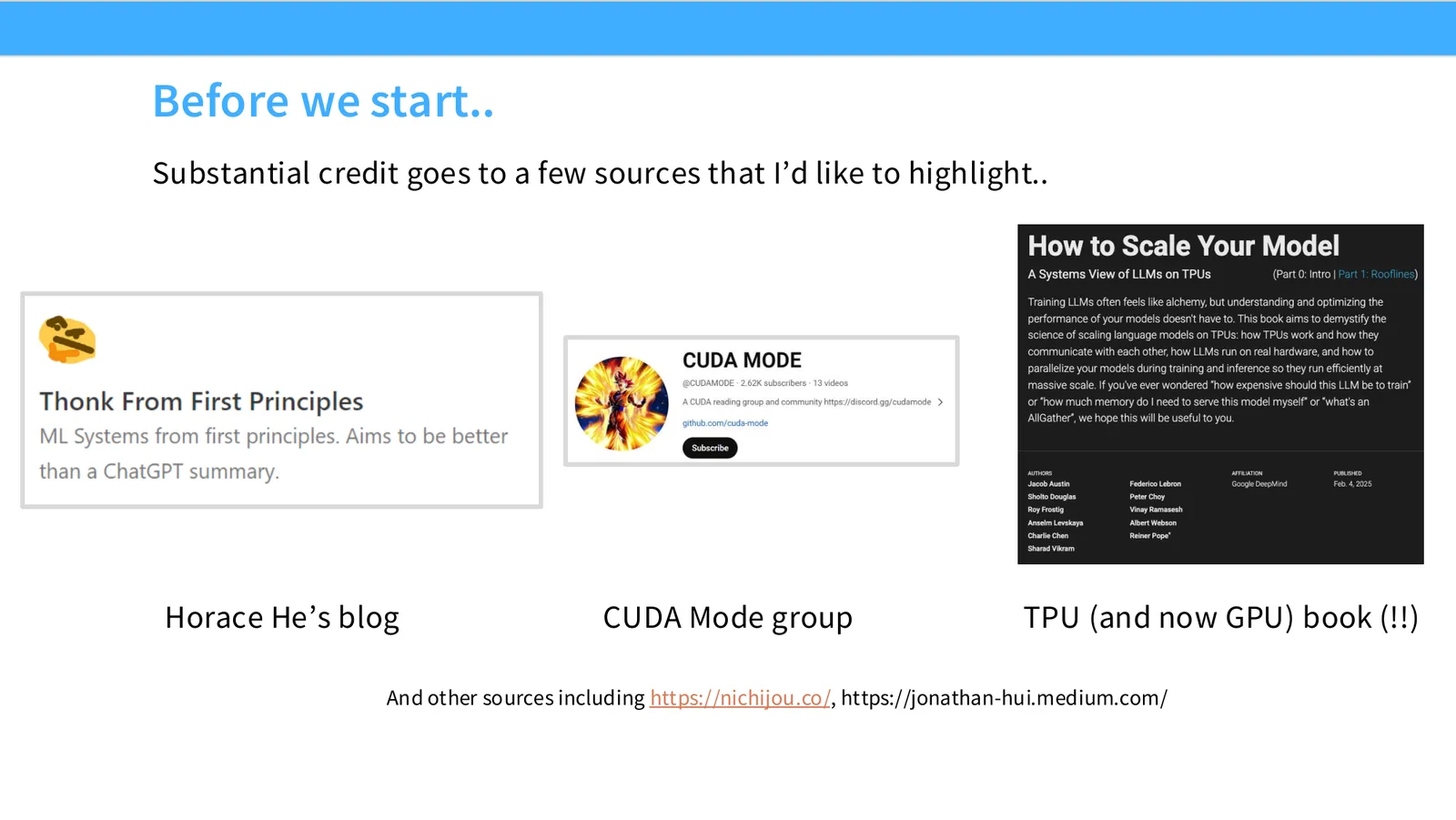
Slide 3 单独列出 Horace He 的博客、CUDA Mode 与 GPU/TPU 性能书等来源。它的教学价值在于说明 GPU performance 是跨层知识:硬件手册给约束,kernel 社区提供实现模式,论文展示 IO-aware algorithm。讲义应保持这些证据层分开——硬件规格不等于实际 kernel 性能,单个 benchmark 也不等于普遍算法规律。
来源:CS336 Spring 2026 Lecture 5 官方幻灯片。
证据层次:spec、microbenchmark、end-to-end
GPU datasheet 告诉我们峰值 FLOP/s、带宽和片上容量;microbenchmark 检查某种 shape、dtype 或访问模式能达到多少;端到端训练则包含 framework dispatch、通信和其他算子。一个优化只有在三层证据一致时才可信:规格上有上限空间,microbenchmark 证明实现接近上限,完整 workload 证明局部收益没有被别处抵消。
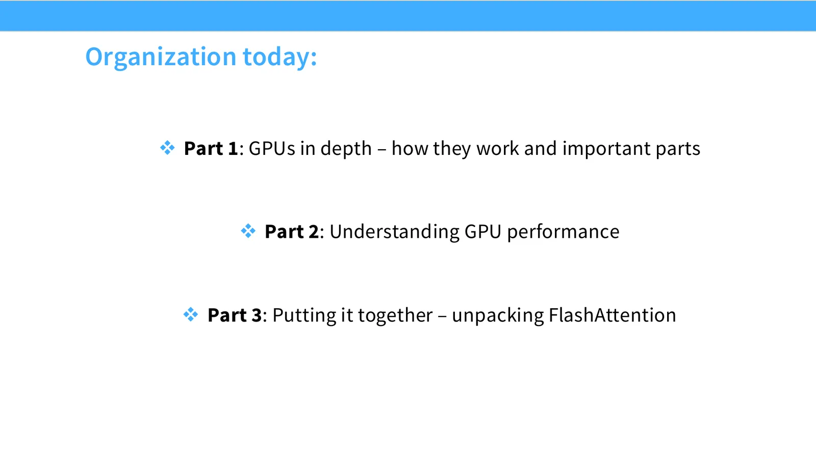
最后的组织页把全讲分成三段:先拆 GPU 硬件与 memory model,再建立 workload performance 技巧,最后用 FlashAttention 验证这些技巧如何组合。这个顺序防止把 FlashAttention 神秘化:其核心组件——tiling、online normalization、避免中间矩阵写回——都来自前两部分已经建立的 IO 账本。
来源:CS336 Spring 2026 Lecture 5 官方幻灯片。
全讲阅读问题
每一页至少回答一个问题:数据当前在 HBM、shared memory 还是 register?并行工作能否填满 SM?矩阵 shape 是否匹配 tensor core tile?减少精度或重算后,节省的 byte 是否大于新增计算?到 FlashAttention 部分时,这四个问题会被放进同一条 forward-pass 数据流。
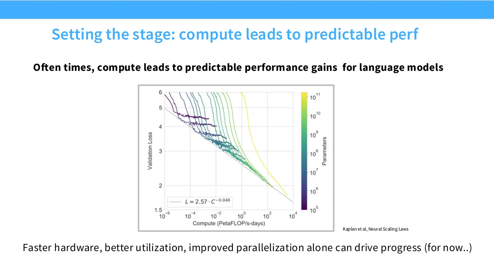
来源:CS336 Spring 2026 Lecture 5 官方幻灯片。
展开说明:Often times, compute leads to predictable performance gains for language models
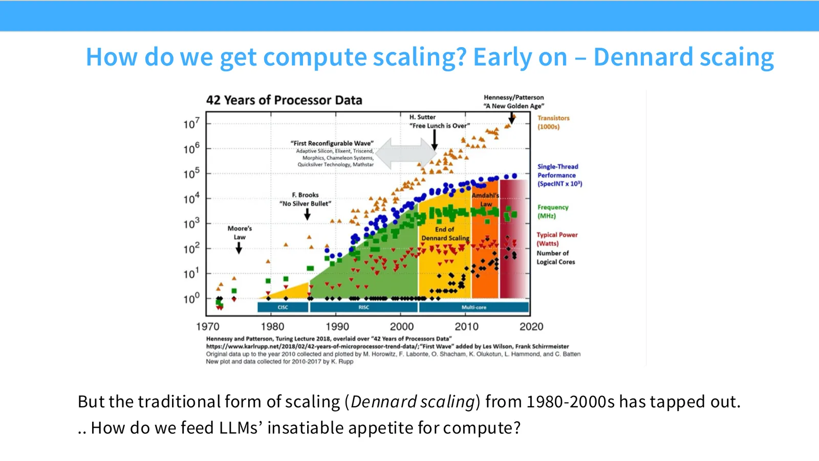
来源:CS336 Spring 2026 Lecture 5 官方幻灯片。
展开说明:But the traditional form of scaling (Dennard scaling) from 1980-2000s has tapped out.
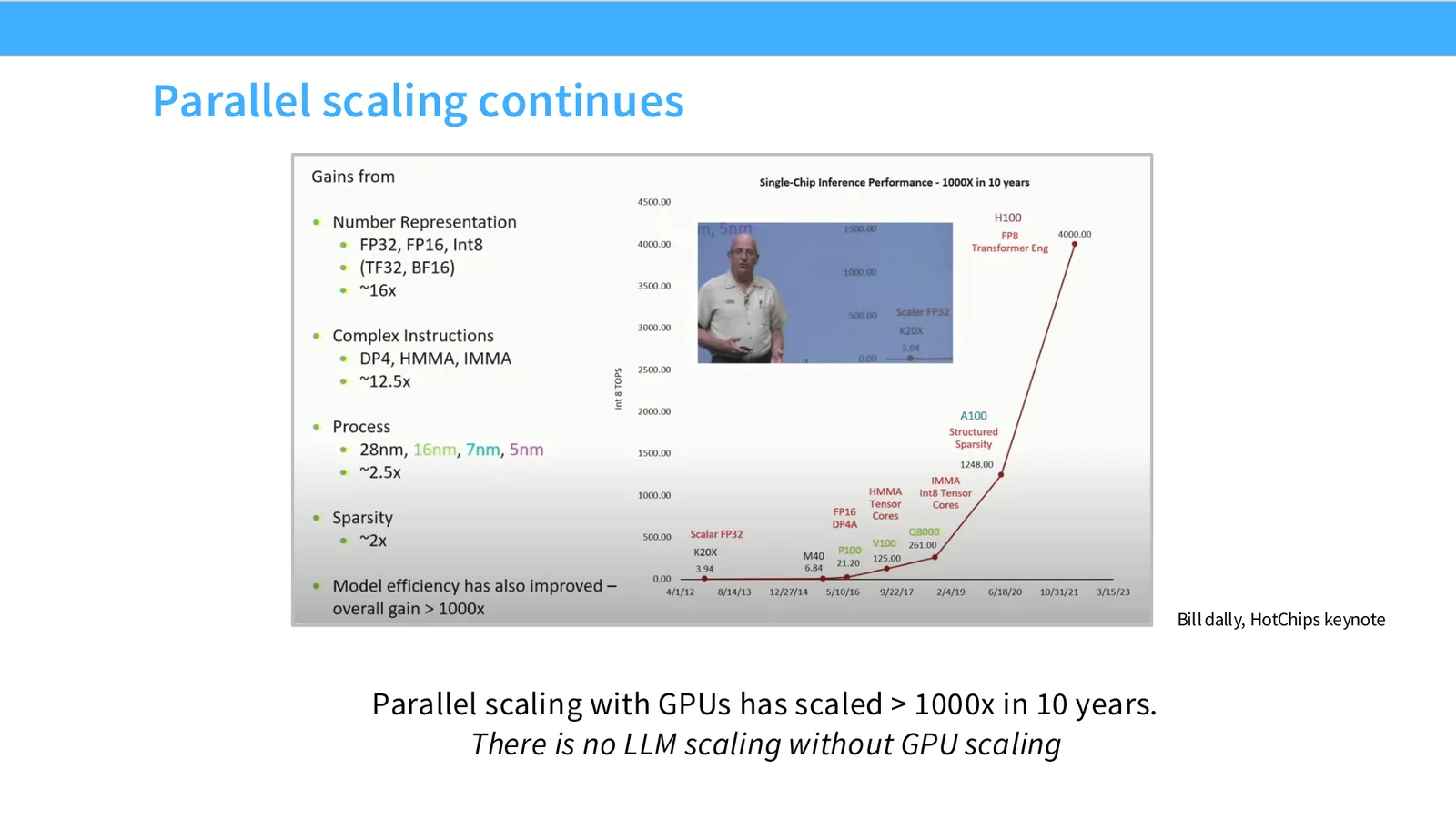
来源:CS336 Spring 2026 Lecture 5 官方幻灯片。
展开说明:Bill dally, HotChips keynote
读图:Slide 7 应该怎么看
这页是硬件机制或性能证据页。先看数据从哪里来、在哪里复用、是否写回 HBM;再判断瓶颈是 compute、memory bandwidth、thread scheduling 还是 alignment。GPU 优化不是让公式更漂亮,而是让数据在正确层级停留更久、让 tensor cores 少等数据。
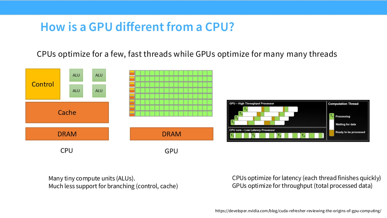
来源:CS336 Spring 2026 Lecture 5 官方幻灯片。
展开说明:CPUs optimize for a few, fast threads while GPUs optimize for many many threads
读图:Slide 8 应该怎么看
这页是硬件机制或性能证据页。先看数据从哪里来、在哪里复用、是否写回 HBM;再判断瓶颈是 compute、memory bandwidth、thread scheduling 还是 alignment。GPU 优化不是让公式更漂亮,而是让数据在正确层级停留更久、让 tensor cores 少等数据。
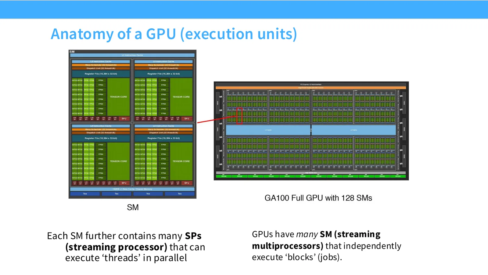
来源:CS336 Spring 2026 Lecture 5 官方幻灯片。
展开说明:Each SM further contains many SPs GPUs have many SM (streaming
读图:Slide 9 应该怎么看
这页是硬件机制或性能证据页。先看数据从哪里来、在哪里复用、是否写回 HBM;再判断瓶颈是 compute、memory bandwidth、thread scheduling 还是 alignment。GPU 优化不是让公式更漂亮,而是让数据在正确层级停留更久、让 tensor cores 少等数据。
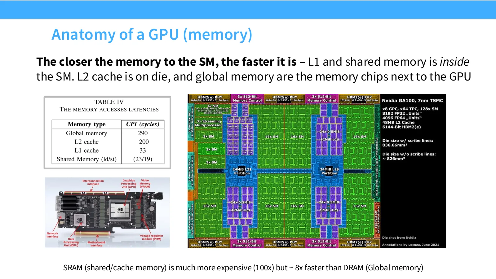
来源:CS336 Spring 2026 Lecture 5 官方幻灯片。
展开说明:The closer the memory to the SM, the faster it is – L1 and shared memory is inside
读图:Slide 10 应该怎么看
这页是硬件机制或性能证据页。先看数据从哪里来、在哪里复用、是否写回 HBM;再判断瓶颈是 compute、memory bandwidth、thread scheduling 还是 alignment。GPU 优化不是让公式更漂亮,而是让数据在正确层级停留更久、让 tensor cores 少等数据。
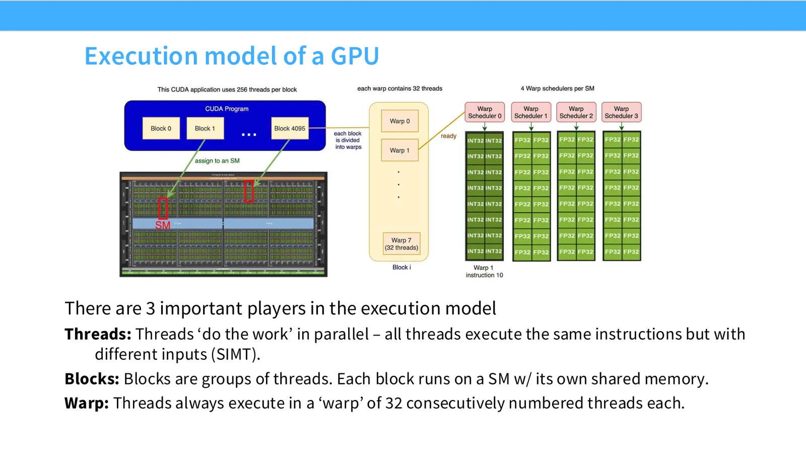
来源:CS336 Spring 2026 Lecture 5 官方幻灯片。
展开说明:There are 3 important players in the execution model
读图:Slide 11 应该怎么看
这页是硬件机制或性能证据页。先看数据从哪里来、在哪里复用、是否写回 HBM;再判断瓶颈是 compute、memory bandwidth、thread scheduling 还是 alignment。GPU 优化不是让公式更漂亮,而是让数据在正确层级停留更久、让 tensor cores 少等数据。
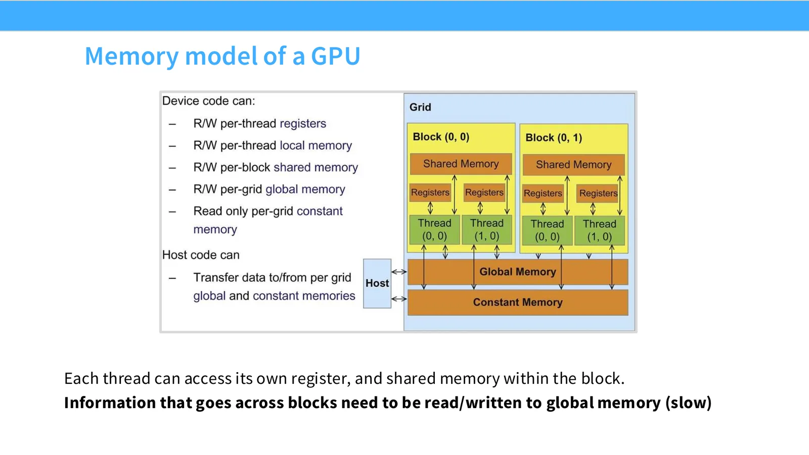
来源:CS336 Spring 2026 Lecture 5 官方幻灯片。
展开说明:Each thread can access its own register, and shared memory within the block.
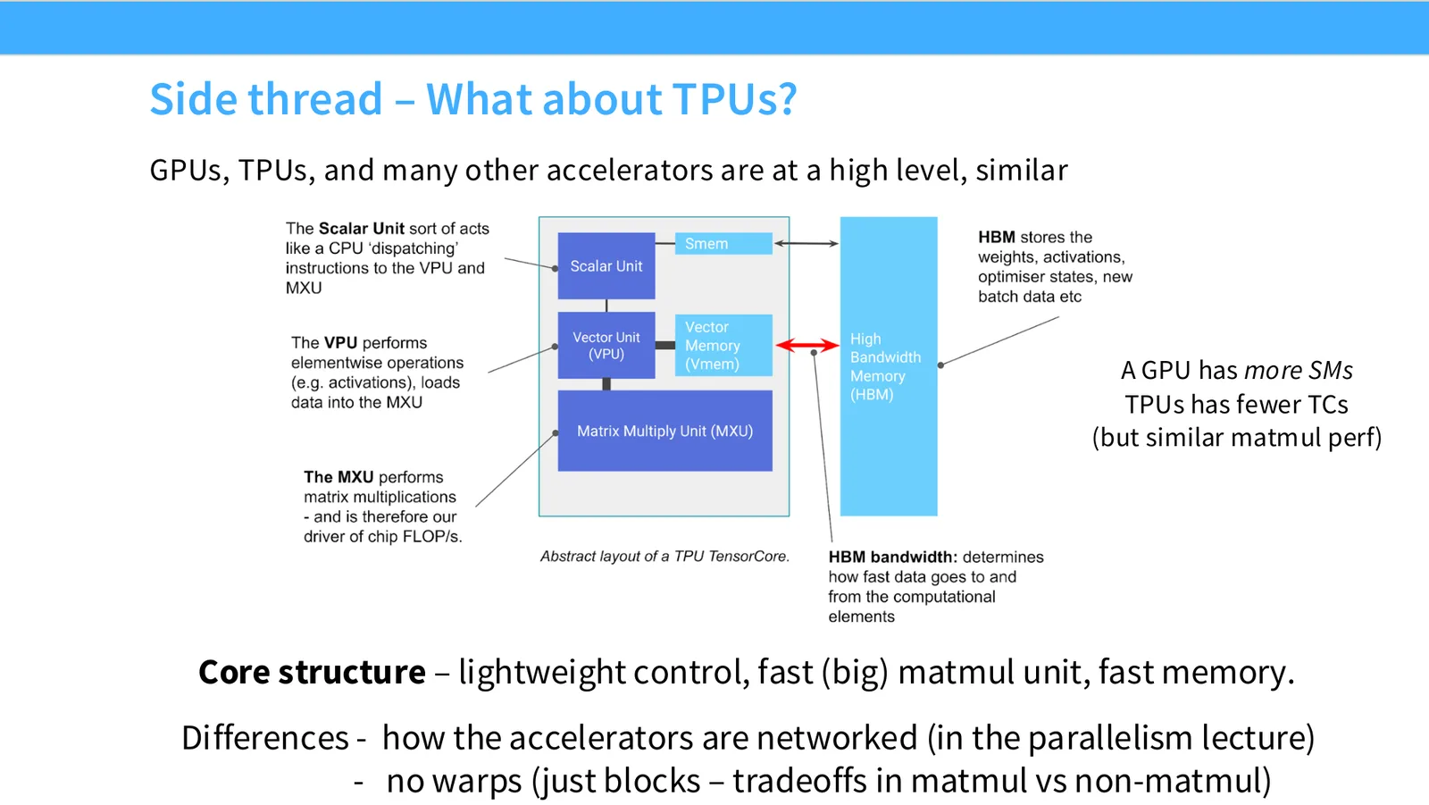
来源:CS336 Spring 2026 Lecture 5 官方幻灯片。
展开说明:GPUs, TPUs, and many other accelerators are at a high level, similar
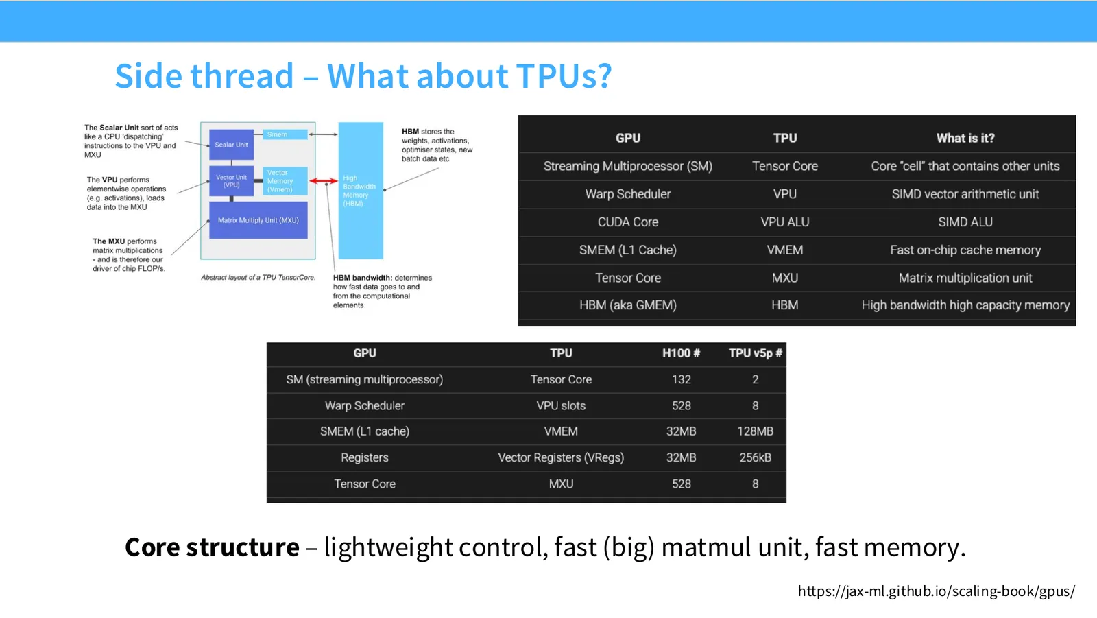
来源:CS336 Spring 2026 Lecture 5 官方幻灯片。
展开说明:Core structure – lightweight control, fast (big) matmul unit, fast memory.
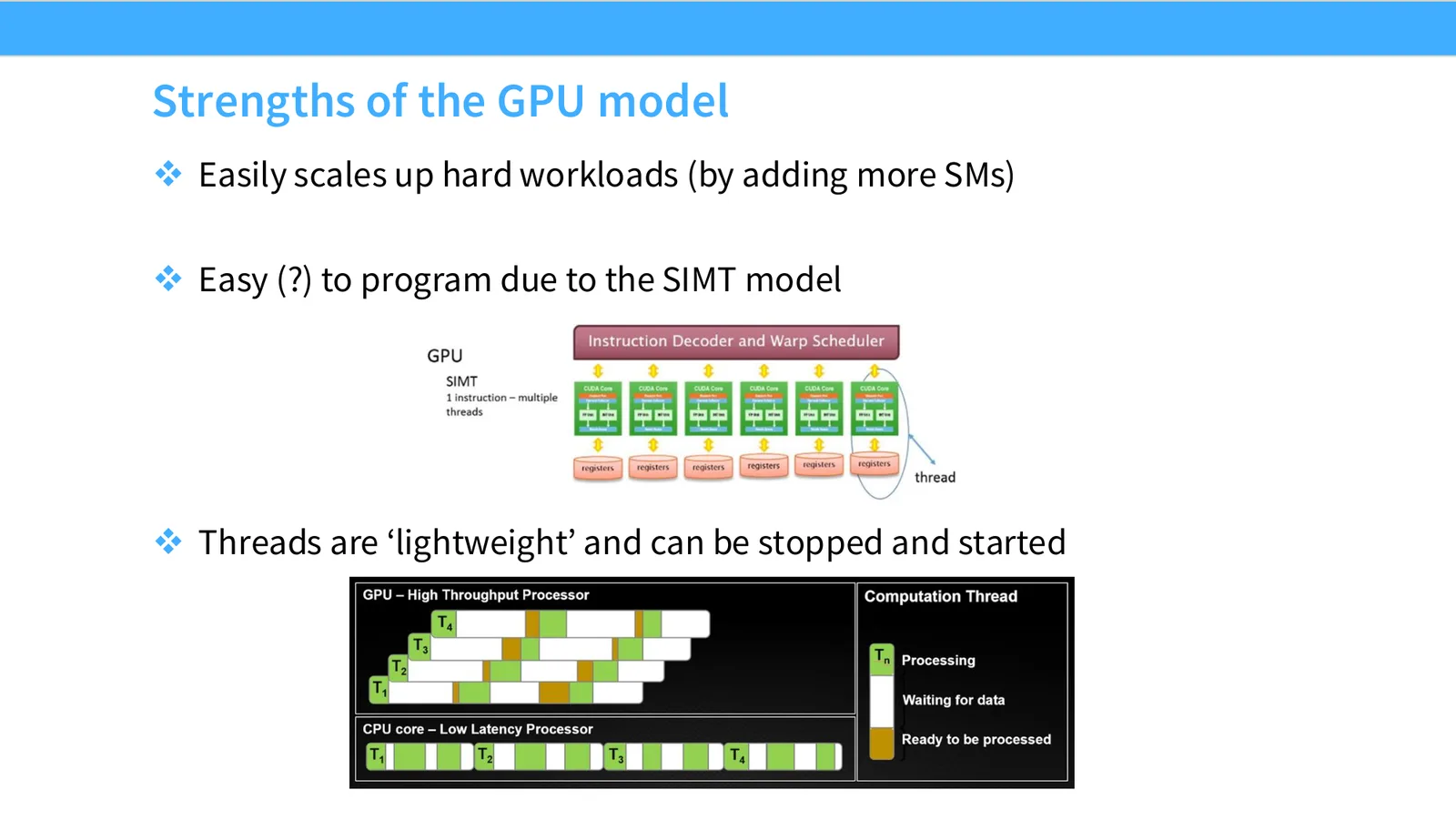
来源:CS336 Spring 2026 Lecture 5 官方幻灯片。
展开说明: Easily scales up hard workloads (by adding more SMs)
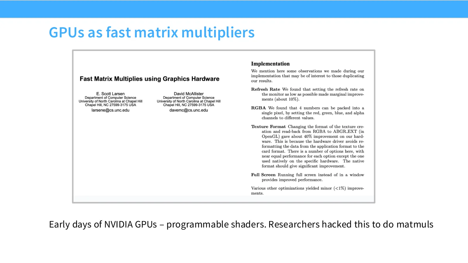
来源:CS336 Spring 2026 Lecture 5 官方幻灯片。
展开说明:Early days of NVIDIA GPUs – programmable shaders. Researchers hacked this to do matmuls
读图:Slide 16 应该怎么看
这页是硬件机制或性能证据页。先看数据从哪里来、在哪里复用、是否写回 HBM;再判断瓶颈是 compute、memory bandwidth、thread scheduling 还是 alignment。GPU 优化不是让公式更漂亮,而是让数据在正确层级停留更久、让 tensor cores 少等数据。
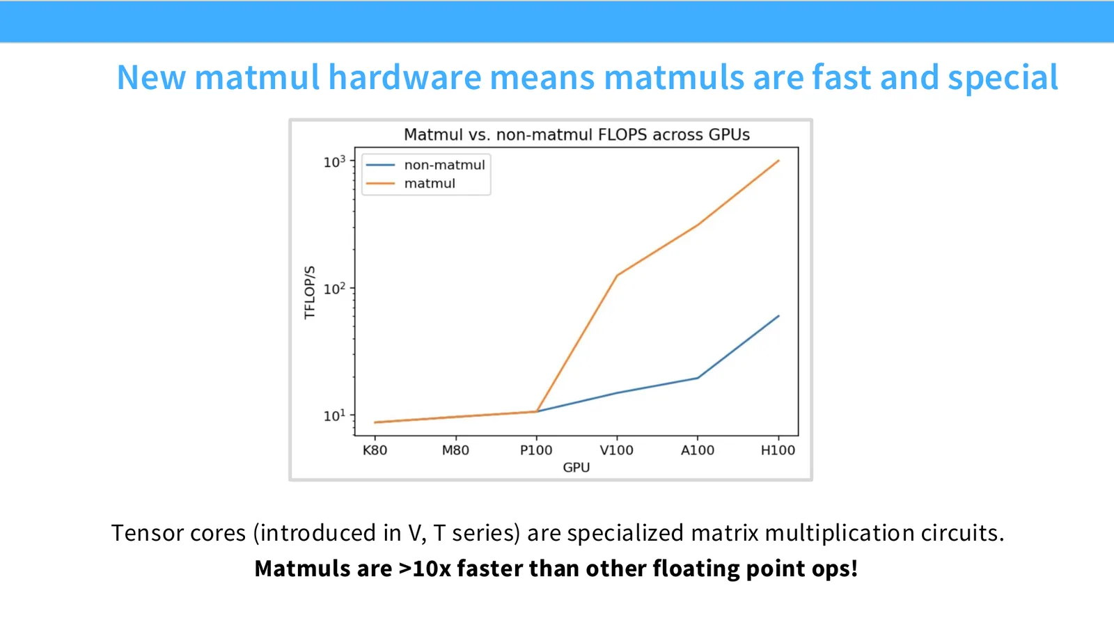
来源:CS336 Spring 2026 Lecture 5 官方幻灯片。
展开说明:Tensor cores (introduced in V, T series) are specialized matrix multiplication circuits.
读图:Slide 17 应该怎么看
这页是硬件机制或性能证据页。先看数据从哪里来、在哪里复用、是否写回 HBM;再判断瓶颈是 compute、memory bandwidth、thread scheduling 还是 alignment。GPU 优化不是让公式更漂亮,而是让数据在正确层级停留更久、让 tensor cores 少等数据。
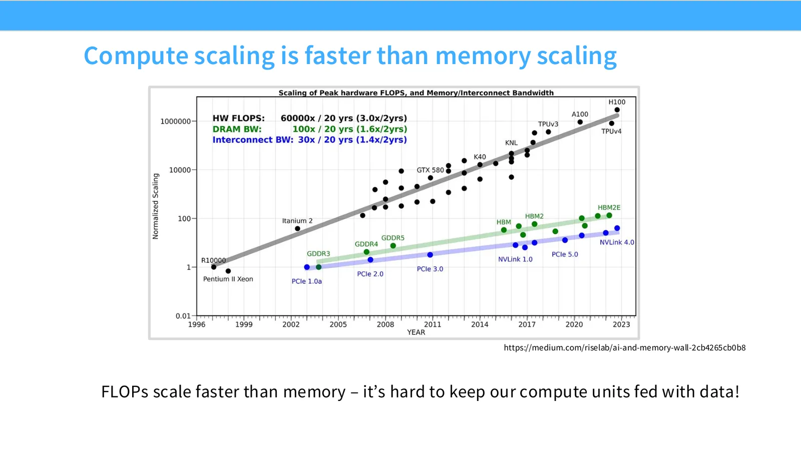
来源:CS336 Spring 2026 Lecture 5 官方幻灯片。
展开说明:https://medium.com/riselab/ai-and-memory-wall-2cb4265cb0b8
前 18 页的硬件事实在 Slide 19 被压缩成三条:GPU 依赖大量 workers 执行相同指令;矩阵计算峰值增长快于 memory;程序必须尊重多层 memory hierarchy。三条缺一不可——只有并行而没有复用会受带宽限制,只有 tensor cores 而 shape 不匹配会受调度限制,只有片上 memory 而 tile 设计错误也无法复用。
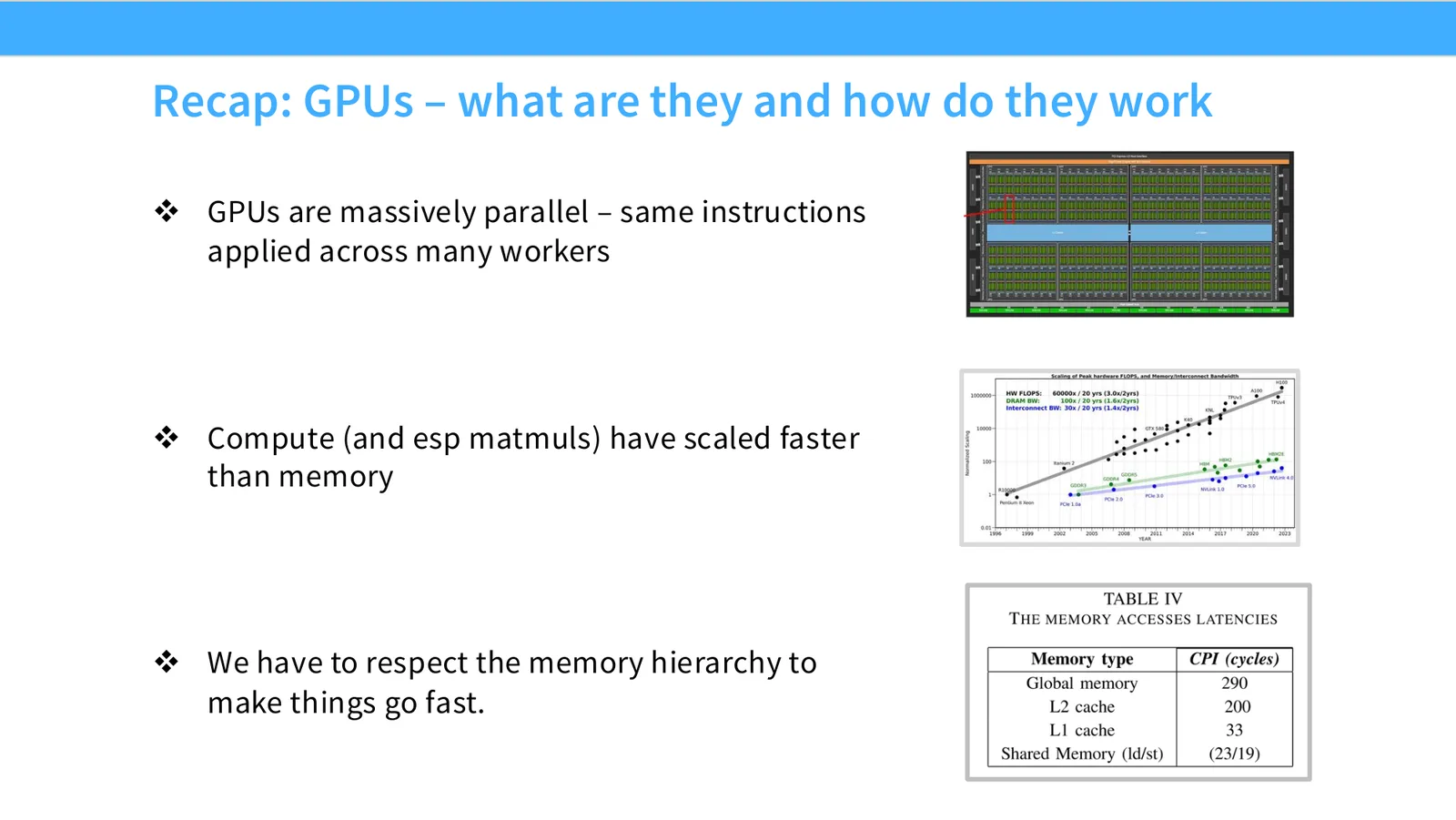
来源:CS336 Spring 2026 Lecture 5 官方幻灯片。
从硬件事实到性能诊断
若 kernel 低于预期,先按三层排查:warp 是否因 divergence 或工作量太小而空闲;arithmetic intensity 是否低到受 HBM bandwidth 限制;数据是否被及时搬到 shared memory/register 并重复使用。后面的低精度、fusion、coalescing 与 tiling 分别作用于这些层,而不是互相替代。
本章小结
本节的共同问题是如何减少昂贵的数据移动并提高硬件利用率。GPU 的速度来自海量并行和专用矩阵硬件,但只有当 memory access、shape、precision 和 kernel 组织匹配时,这些速度才会真正出现。
Roofline 与低精度:让 ML workload 跑快
前一节已经说明 GPU 的峰值计算增长快于 memory bandwidth;本节把这个硬件事实转成 workload 性能模型。我们先用 roofline 判断算子是 compute-bound 还是 memory-bound,再区分 divergence、低并行度与 memory traffic,最后检查 FP8、MXFP8、MXFP4 如何同时改变 bytes moved、tensor-core throughput 和数值误差。读后续曲线时应先定位瓶颈,再讨论某种 dtype 或 kernel 是否真的解决了它。
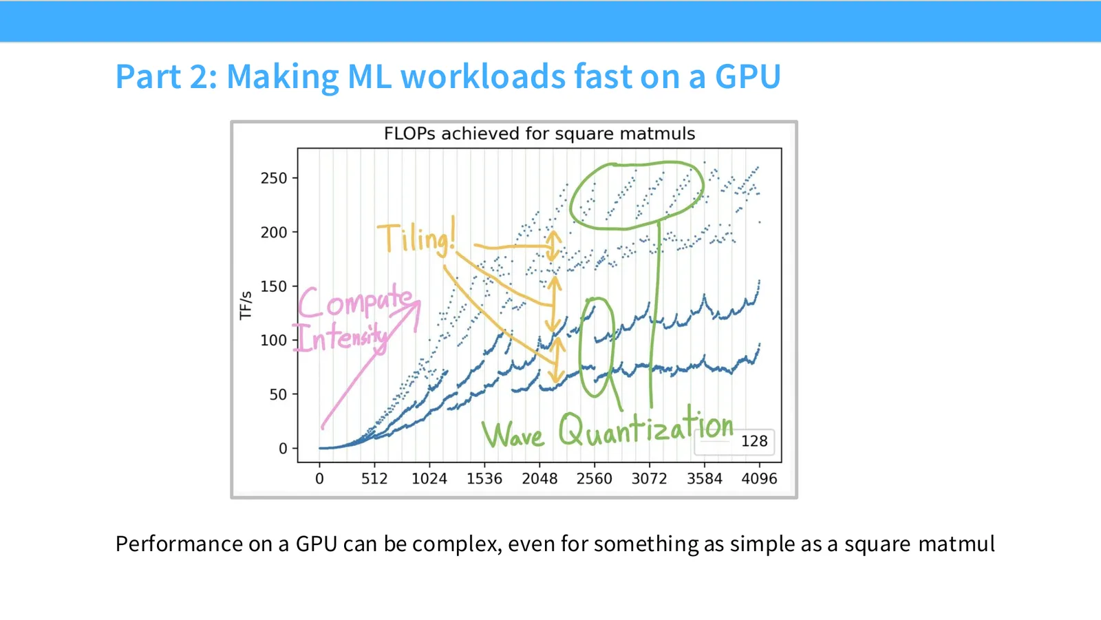
来源:CS336 Spring 2026 Lecture 5 官方幻灯片。
为什么简单 matmul 也不平滑
同样的 \(n^3\) FLOPs 不会带来平滑 runtime:矩阵维度会影响 tile 对齐、可并发 thread blocks、wave 数量、cache 行为与 tensor core kernel 选择。性能曲线中的锯齿或周期性通常不是测量噪声,而是离散硬件资源被整除或留下尾部 wave;后面的 matrix mystery 会用 tiling 与 wave quantization 解释。
性能公式:roofline 心智模型
低精度减少 bytes moved,也可能启用 tensor cores,因此同时影响 memory traffic 和 peak compute。
展开说明: GPUs are massively parallel – same instructions
展开说明:Performance on a GPU can be complex, even for something as simple as a square matmul
讲义补充:源 Slide 20 应该怎么看
这页是硬件机制或性能证据页。先看数据从哪里来、在哪里复用、是否写回 HBM;再判断瓶颈是 compute、memory bandwidth、thread scheduling 还是 alignment。GPU 优化不是让公式更漂亮,而是让数据在正确层级停留更久、让 tensor cores 少等数据。
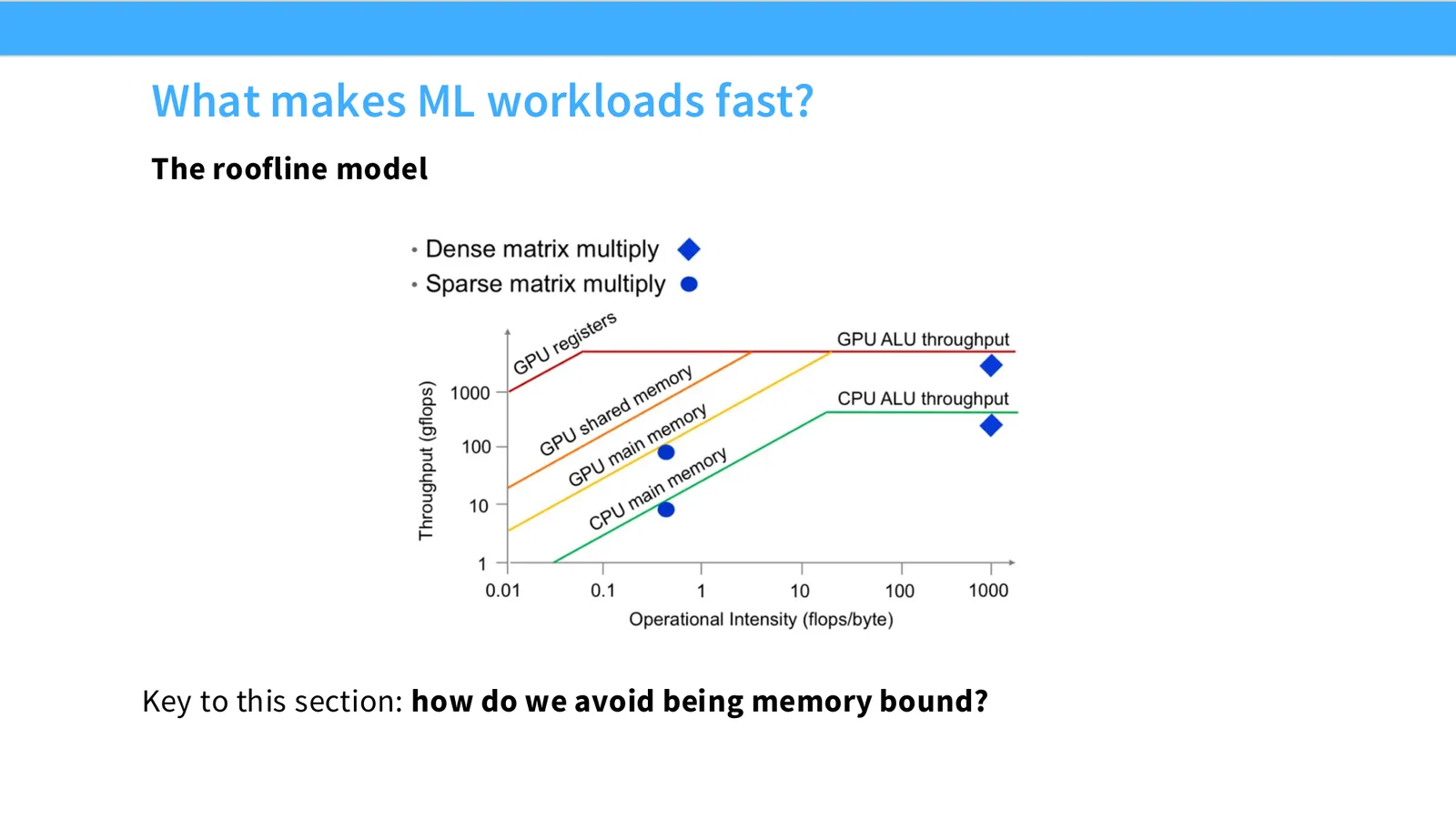
来源:CS336 Spring 2026 Lecture 5 官方幻灯片。
展开说明:The roofline model
读图:Slide 21 应该怎么看
这页是硬件机制或性能证据页。先看数据从哪里来、在哪里复用、是否写回 HBM;再判断瓶颈是 compute、memory bandwidth、thread scheduling 还是 alignment。GPU 优化不是让公式更漂亮,而是让数据在正确层级停留更久、让 tensor cores 少等数据。
Roofline 给出统一上限后,Slide 22 把优化手段列成六项:控制 divergence、低精度、operator fusion、recomputation、coalescing 与 tiling。列表本身不是按固定优先级执行的 recipe,而是 bottleneck 到动作的映射:divergence 修复执行单元空转;低精度同时减少 byte 并提高 tensor-core 峰值;其余四项主要减少或重排 memory traffic。
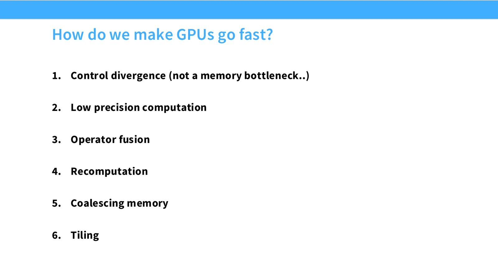
来源:CS336 Spring 2026 Lecture 5 官方幻灯片。
先测瓶颈,再选技巧
Memory-bound elementwise chain 优先 fusion;重复读取大张量可考虑 recomputation;跨 thread 的连续访问不佳时检查 coalescing;矩阵数据不能在片上复用时做 tiling;warp 内分支不同才处理 divergence。若 kernel 已 compute-bound,继续减少 HBM 访问可能没有收益,此时应看 precision、tensor-core tile 和 occupancy。
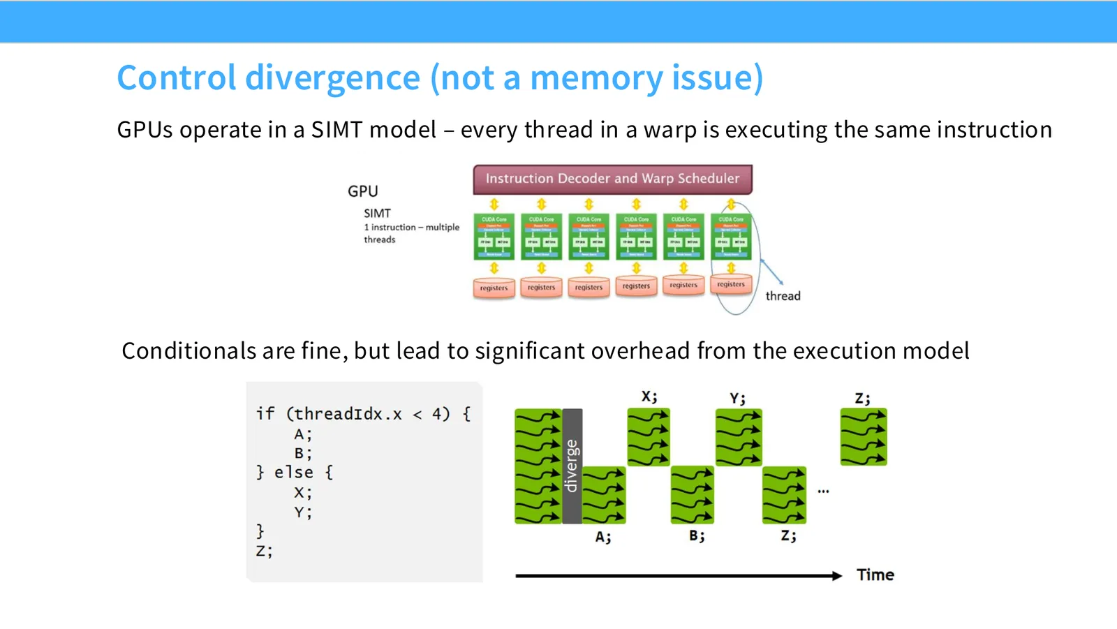
来源:CS336 Spring 2026 Lecture 5 官方幻灯片。
展开说明:GPUs operate in a SIMT model – every thread in a warp is executing the same instruction
读图:Slide 23 应该怎么看
这页是硬件机制或性能证据页。先看数据从哪里来、在哪里复用、是否写回 HBM;再判断瓶颈是 compute、memory bandwidth、thread scheduling 还是 alignment。GPU 优化不是让公式更漂亮,而是让数据在正确层级停留更久、让 tensor cores 少等数据。
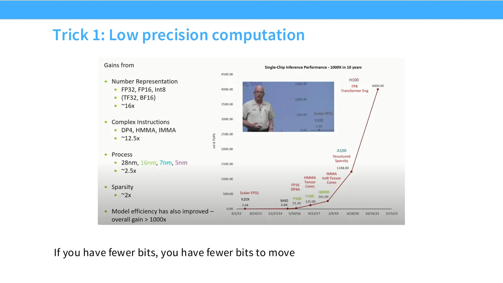
来源:CS336 Spring 2026 Lecture 5 官方幻灯片。
展开说明:If you have fewer bits, you have fewer bits to move
读图:Slide 24 应该怎么看
这页是硬件机制或性能证据页。先看数据从哪里来、在哪里复用、是否写回 HBM;再判断瓶颈是 compute、memory bandwidth、thread scheduling 还是 alignment。GPU 优化不是让公式更漂亮,而是让数据在正确层级停留更久、让 tensor cores 少等数据。
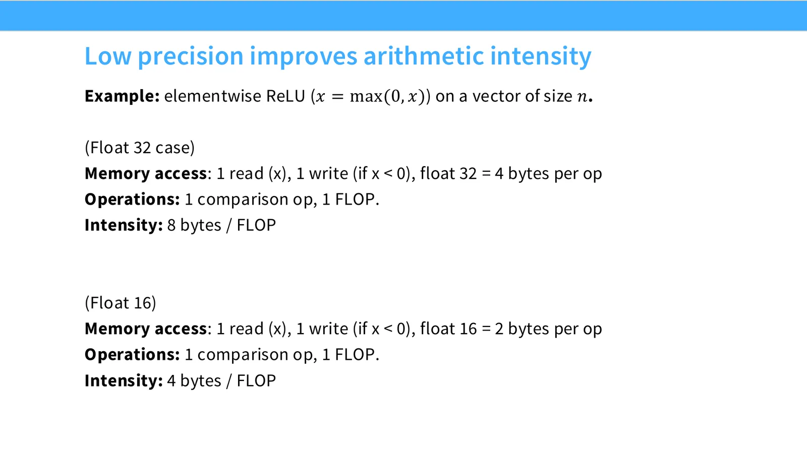
来源:CS336 Spring 2026 Lecture 5 官方幻灯片。
展开说明:Example: elementwise ReLU (\(x\) = max(0, \(x\))) on a vector of size \(n\).
读图:Slide 25 应该怎么看
这页是硬件机制或性能证据页。先看数据从哪里来、在哪里复用、是否写回 HBM;再判断瓶颈是 compute、memory bandwidth、thread scheduling 还是 alignment。GPU 优化不是让公式更漂亮,而是让数据在正确层级停留更久、让 tensor cores 少等数据。
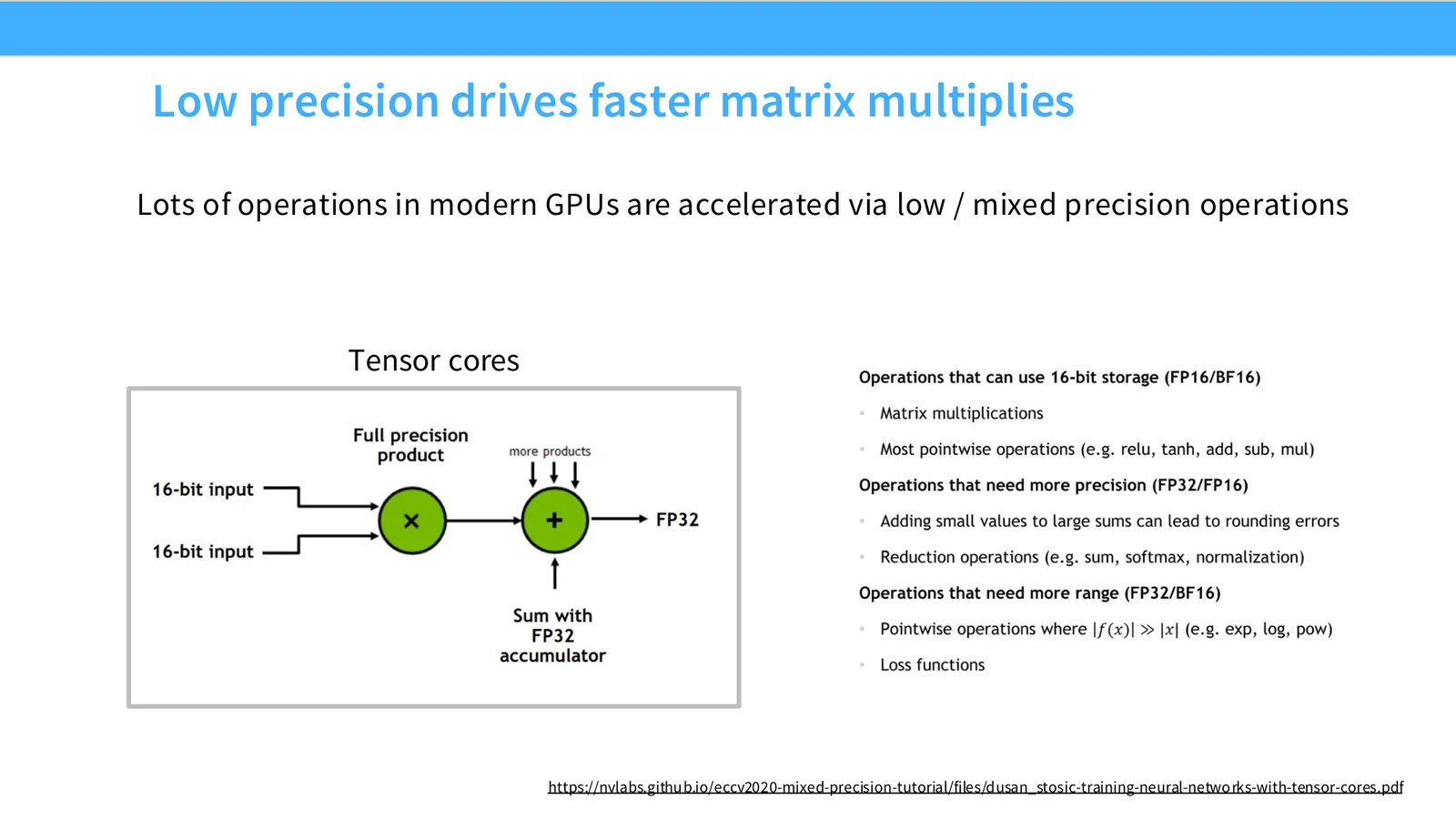
来源:CS336 Spring 2026 Lecture 5 官方幻灯片。
展开说明:Lots of operations in modern GPUs are accelerated via low / mixed precision operations
读图:Slide 26 应该怎么看
这页是硬件机制或性能证据页。先看数据从哪里来、在哪里复用、是否写回 HBM;再判断瓶颈是 compute、memory bandwidth、thread scheduling 还是 alignment。GPU 优化不是让公式更漂亮,而是让数据在正确层级停留更久、让 tensor cores 少等数据。
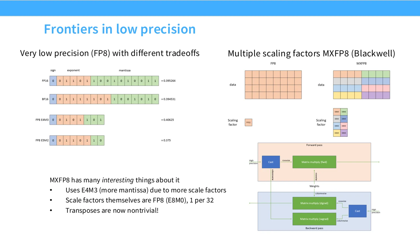
来源:CS336 Spring 2026 Lecture 5 官方幻灯片。
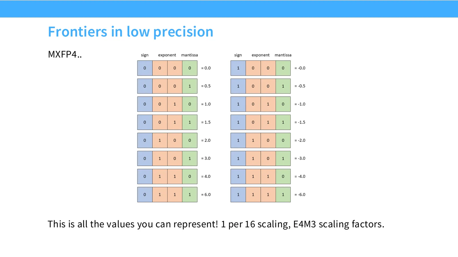
展开说明:Very low precision (FP8) with different tradeoffs Multiple scaling factors MXFP8 (Blackwell)
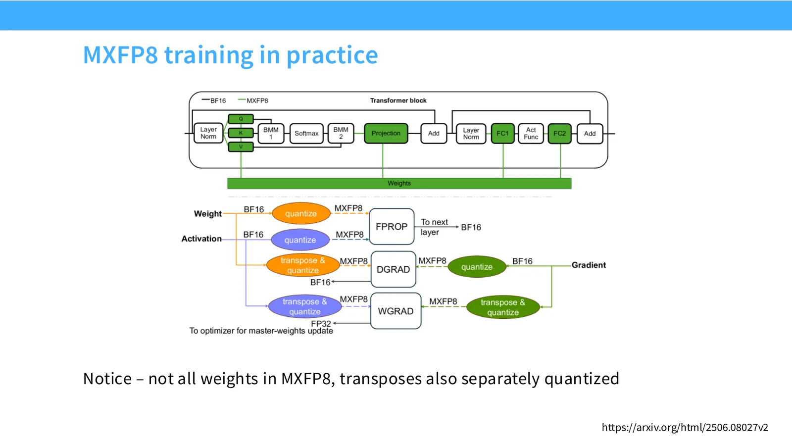
来源:CS336 Spring 2026 Lecture 5 官方幻灯片。
展开说明:Notice – not all weights in MXFP8, transposes also separately quantized
低精度部分最后进入 MXFP4。Slide 29 直接展示 4-bit 格式可表示的离散值与每组 scaling factor:位数减少提高吞吐与 arithmetic intensity,却让 dynamic range 和量化误差更敏感。分组 scale 越细,表示更准确,但 scale metadata、转换 kernel 与布局复杂度也更高;训练 recipe 还需要决定哪些权重、activation、gradient 或 transpose 保留更高精度。
来源:CS336 Spring 2026 Lecture 5 官方幻灯片。
低精度收益不能只看 bit 数
FP4 相比 FP8 理论上进一步减半 bytes,但实际速度还取决于硬件原生支持、scale 读取、quantize/dequantize、accumulator precision 和矩阵 shape。若额外转换或 fallback kernel 主导,4-bit 可能比成熟 FP8 路径更慢;若 scale 过粗,又可能用更多训练 step 才达到同一 loss。验收必须同时报告吞吐、收敛曲线和溢出/饱和统计。
本章小结
本节的共同问题是如何减少昂贵的数据移动并提高硬件利用率。GPU 的速度来自海量并行和专用矩阵硬件,但只有当 memory access、shape、precision 和 kernel 组织匹配时,这些速度才会真正出现。
Operator fusion 与 recomputation:少搬数据
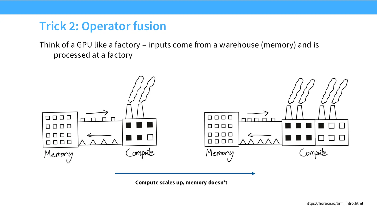
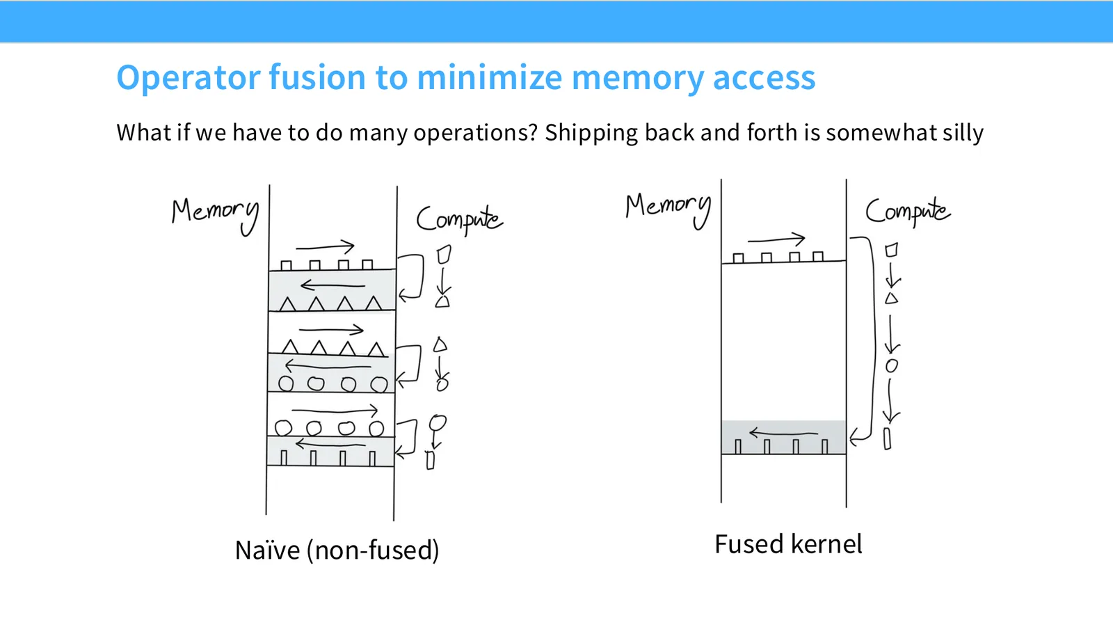
本节用工厂/仓库类比说明 HBM 往返为什么贵,再解释 fusion 和 recomputation 如何减少 memory access。
first-use glossary:operator fusion 与 recomputation
Operator fusion 把多个小 kernel 合成一个 kernel,让中间结果留在寄存器/shared memory 中,减少 HBM 读写。Recomputation 是丢弃某些中间 activations,在需要时重算,用额外 compute 换更低 memory traffic 或 peak memory。
这张 MXFP4 页也完成了第二部分到 operator fusion 的过渡:降低单元素 byte 只是减少 traffic 的一种方法,另一种方法是根本不把中间结果写回 HBM。于是下一节从“每次搬更少”转向“减少搬运次数”,比较 fusion 与 recomputation 如何改变 kernel 边界和 activation 生命周期。
讲义补充:源 Slide 29 应该怎么看
这页是硬件机制或性能证据页。先看数据从哪里来、在哪里复用、是否写回 HBM;再判断瓶颈是 compute、memory bandwidth、thread scheduling 还是 alignment。GPU 优化不是让公式更漂亮,而是让数据在正确层级停留更久、让 tensor cores 少等数据。
来源:CS336 Spring 2026 Lecture 5 官方幻灯片。
展开说明:Think of a GPU like a factory – inputs come from a warehouse (memory) and is
读图:Slide 30 应该怎么看
这页是硬件机制或性能证据页。先看数据从哪里来、在哪里复用、是否写回 HBM;再判断瓶颈是 compute、memory bandwidth、thread scheduling 还是 alignment。GPU 优化不是让公式更漂亮,而是让数据在正确层级停留更久、让 tensor cores 少等数据。
来源:CS336 Spring 2026 Lecture 5 官方幻灯片。
展开说明:What if we have to do many operations? Shipping back and forth is somewhat silly
读图:Slide 31 应该怎么看
这页是硬件机制或性能证据页。先看数据从哪里来、在哪里复用、是否写回 HBM;再判断瓶颈是 compute、memory bandwidth、thread scheduling 还是 alignment。GPU 优化不是让公式更漂亮,而是让数据在正确层级停留更久、让 tensor cores 少等数据。
来源:CS336 Spring 2026 Lecture 5 官方幻灯片。
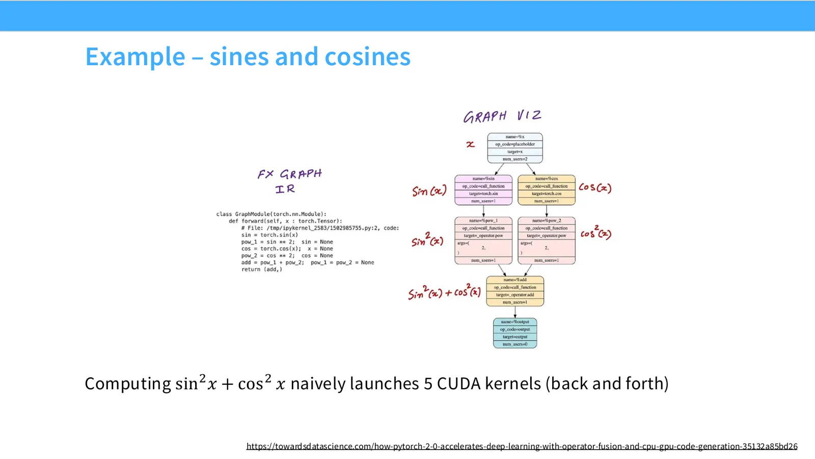
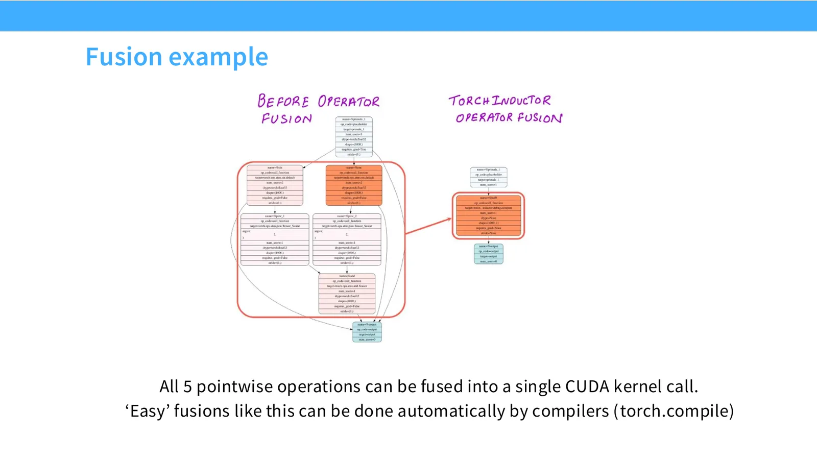
展开说明:Computing sin 2 \(x\) + cos 2 \(x\) naively launches 5 CUDA kernels (back and forth)
读图:Slide 32 应该怎么看
这页是硬件机制或性能证据页。先看数据从哪里来、在哪里复用、是否写回 HBM;再判断瓶颈是 compute、memory bandwidth、thread scheduling 还是 alignment。GPU 优化不是让公式更漂亮,而是让数据在正确层级停留更久、让 tensor cores 少等数据。
来源:CS336 Spring 2026 Lecture 5 官方幻灯片。
展开说明:All 5 pointwise operations can be fused into a single CUDA kernel call.
来源:CS336 Spring 2026 Lecture 5 官方幻灯片。
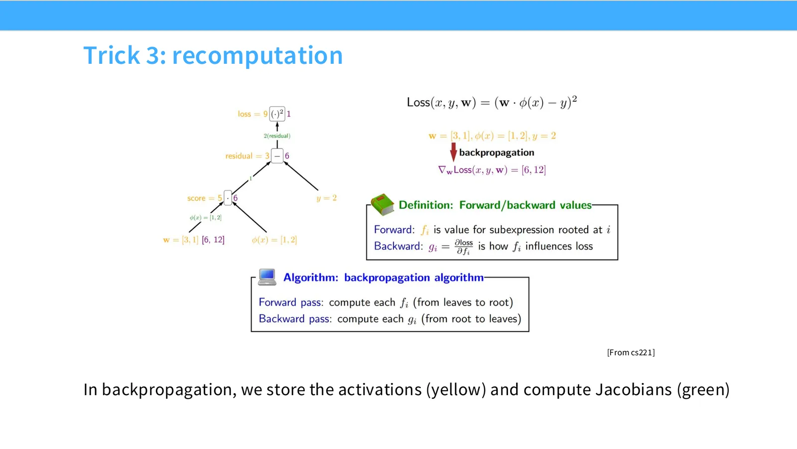
展开说明:[From cs221]
读图:Slide 34 应该怎么看
这页是硬件机制或性能证据页。先看数据从哪里来、在哪里复用、是否写回 HBM;再判断瓶颈是 compute、memory bandwidth、thread scheduling 还是 alignment。GPU 优化不是让公式更漂亮,而是让数据在正确层级停留更久、让 tensor cores 少等数据。
来源:CS336 Spring 2026 Lecture 5 官方幻灯片。
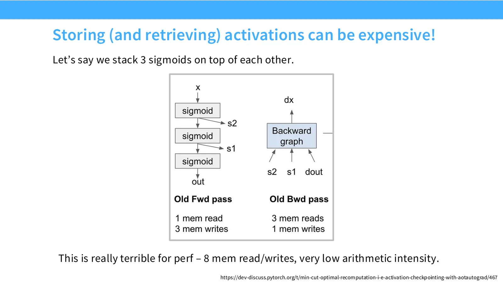
展开说明:Let’s say we stack 3 sigmoids on top of each other.
读图:Slide 35 应该怎么看
这页是硬件机制或性能证据页。先看数据从哪里来、在哪里复用、是否写回 HBM;再判断瓶颈是 compute、memory bandwidth、thread scheduling 还是 alignment。GPU 优化不是让公式更漂亮,而是让数据在正确层级停留更久、让 tensor cores 少等数据。
本章小结
本节的共同问题是如何减少昂贵的数据移动并提高硬件利用率。GPU 的速度来自海量并行和专用矩阵硬件,但只有当 memory access、shape、precision 和 kernel 组织匹配时,这些速度才会真正出现。
Coalescing、tiling 与矩阵性能异常
本节解释 DRAM burst、memory coalescing、row-major matmul、tiling、alignment、wave quantization 和 matrix mystery。
first-use glossary:coalescing、tiling、wave quantization
Memory coalescing 指同一个 warp 的 memory accesses 落在连续 burst 中,从而合并成高效访问。Tiling 把大矩阵切成小块放入 shared memory 重复使用。Wave quantization 指 thread blocks 数量不能完美填满 SM waves 时产生的周期性利用率波动。
来源:CS336 Spring 2026 Lecture 5 官方幻灯片。
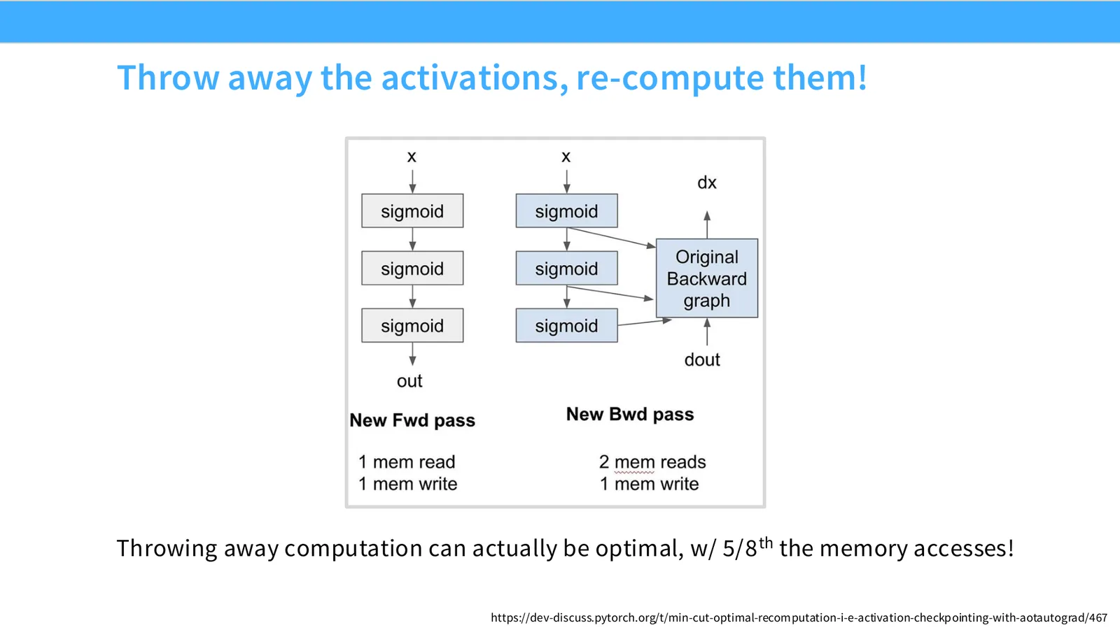
展开说明:Throwing away computation can actually be optimal, w/ 5/8 th the memory accesses!
读图:Slide 36 应该怎么看
这页是硬件机制或性能证据页。先看数据从哪里来、在哪里复用、是否写回 HBM;再判断瓶颈是 compute、memory bandwidth、thread scheduling 还是 alignment。GPU 优化不是让公式更漂亮,而是让数据在正确层级停留更久、让 tensor cores 少等数据。
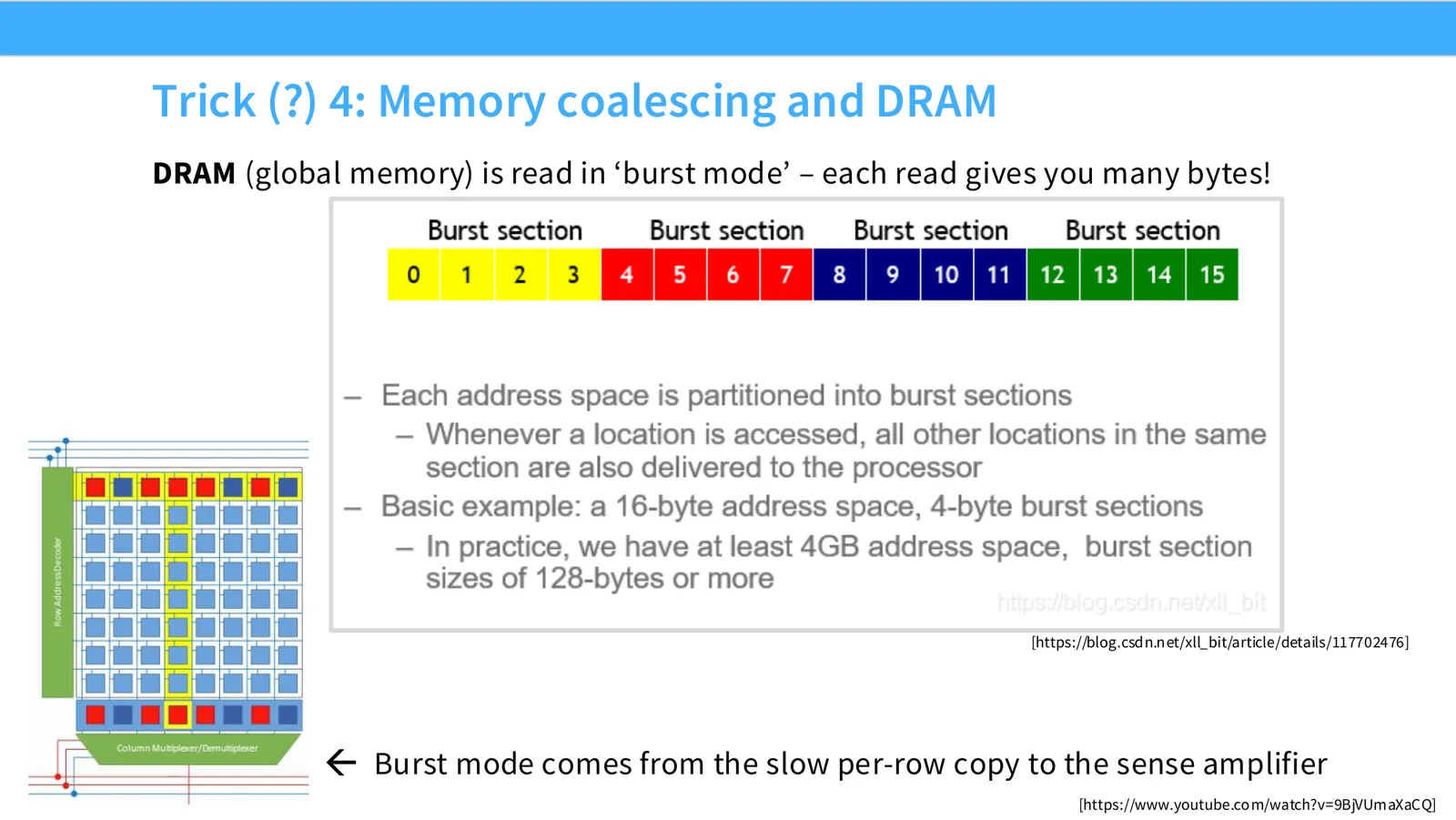
来源:CS336 Spring 2026 Lecture 5 官方幻灯片。
展开说明:DRAM (global memory) is read in ‘burst mode’ – each read gives you many bytes!
读图:Slide 37 应该怎么看
这页是硬件机制或性能证据页。先看数据从哪里来、在哪里复用、是否写回 HBM;再判断瓶颈是 compute、memory bandwidth、thread scheduling 还是 alignment。GPU 优化不是让公式更漂亮,而是让数据在正确层级停留更久、让 tensor cores 少等数据。
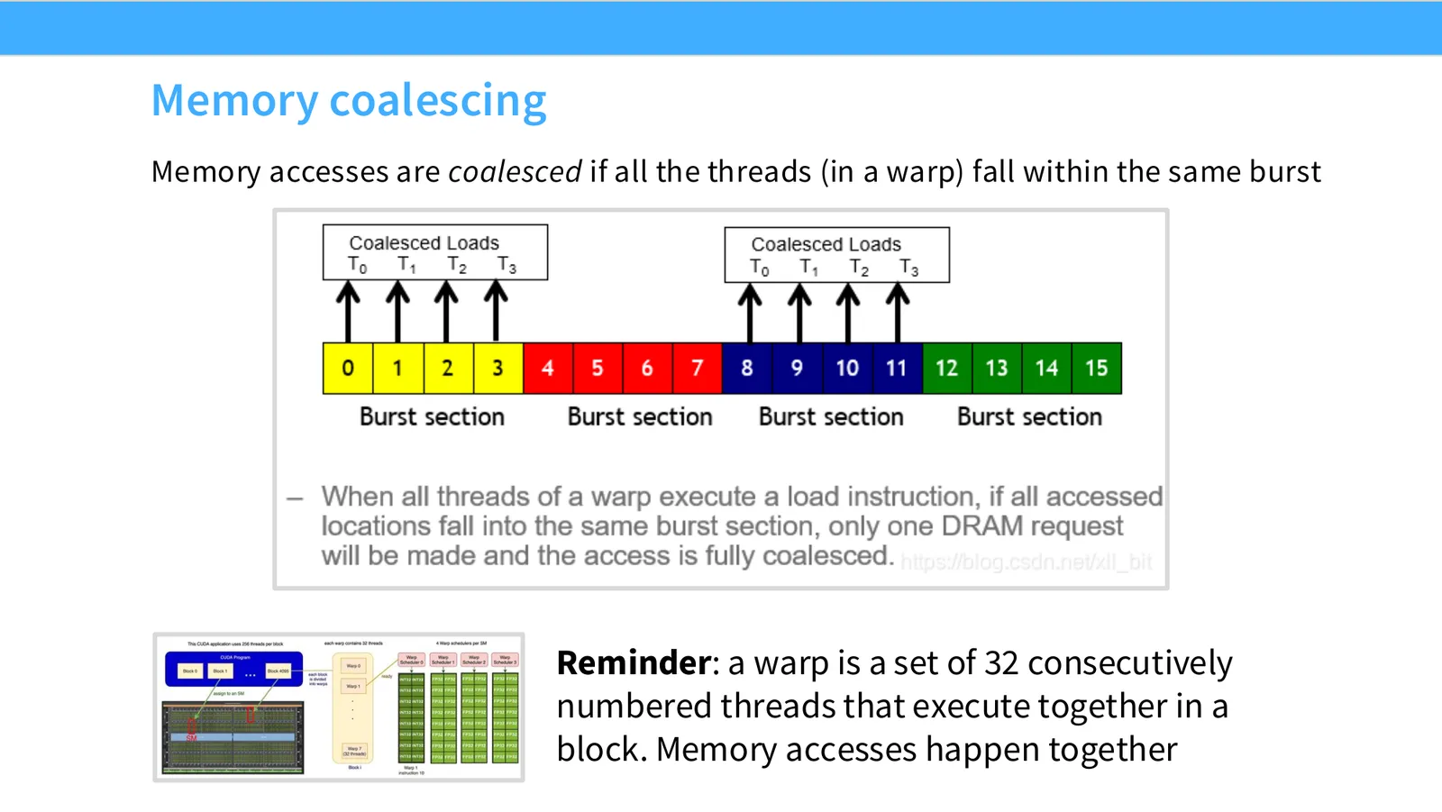
来源:CS336 Spring 2026 Lecture 5 官方幻灯片。
展开说明:Memory accesses are coalesced if all the threads (in a warp) fall within the same burst
读图:Slide 38 应该怎么看
这页是硬件机制或性能证据页。先看数据从哪里来、在哪里复用、是否写回 HBM;再判断瓶颈是 compute、memory bandwidth、thread scheduling 还是 alignment。GPU 优化不是让公式更漂亮,而是让数据在正确层级停留更久、让 tensor cores 少等数据。
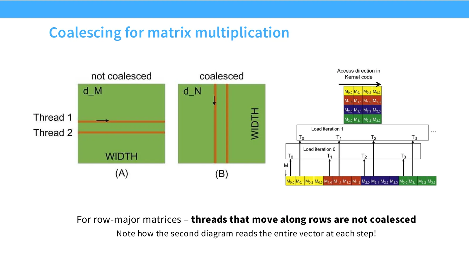
来源:CS336 Spring 2026 Lecture 5 官方幻灯片。
展开说明:For row-major matrices – threads that move along rows are not coalesced
读图:Slide 39 应该怎么看
这页是硬件机制或性能证据页。先看数据从哪里来、在哪里复用、是否写回 HBM;再判断瓶颈是 compute、memory bandwidth、thread scheduling 还是 alignment。GPU 优化不是让公式更漂亮,而是让数据在正确层级停留更久、让 tensor cores 少等数据。
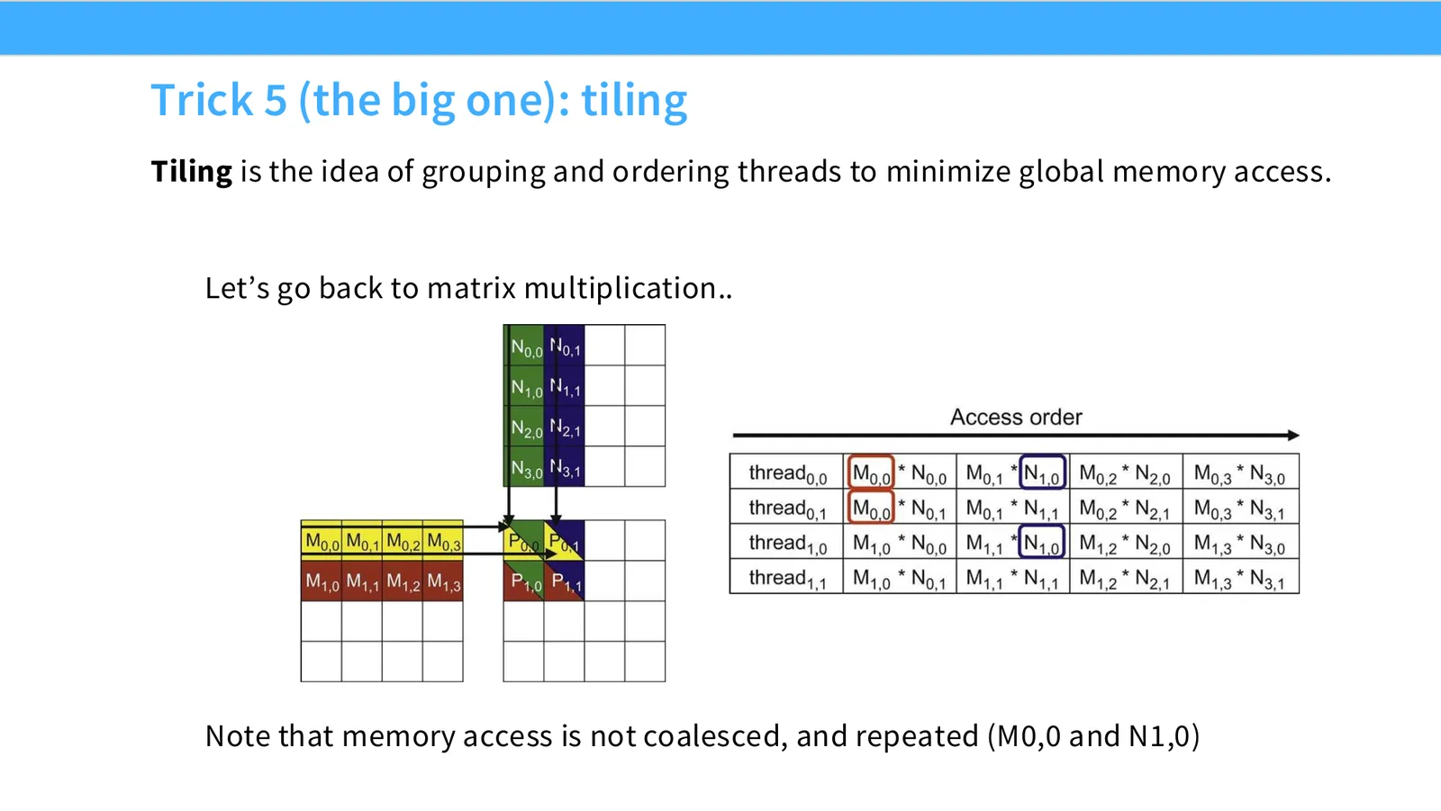
来源:CS336 Spring 2026 Lecture 5 官方幻灯片。
展开说明:Tiling is the idea of grouping and ordering threads to minimize global memory access.
读图:Slide 40 应该怎么看
这页是硬件机制或性能证据页。先看数据从哪里来、在哪里复用、是否写回 HBM;再判断瓶颈是 compute、memory bandwidth、thread scheduling 还是 alignment。GPU 优化不是让公式更漂亮,而是让数据在正确层级停留更久、让 tensor cores 少等数据。
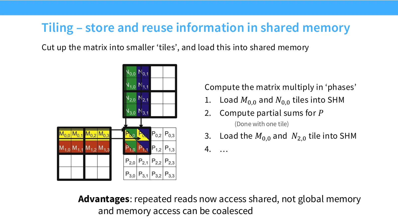
来源:CS336 Spring 2026 Lecture 5 官方幻灯片。
展开说明:Cut up the matrix into smaller ‘tiles’, and load this into shared memory
读图:Slide 41 应该怎么看
这页是硬件机制或性能证据页。先看数据从哪里来、在哪里复用、是否写回 HBM;再判断瓶颈是 compute、memory bandwidth、thread scheduling 还是 alignment。GPU 优化不是让公式更漂亮,而是让数据在正确层级停留更久、让 tensor cores 少等数据。
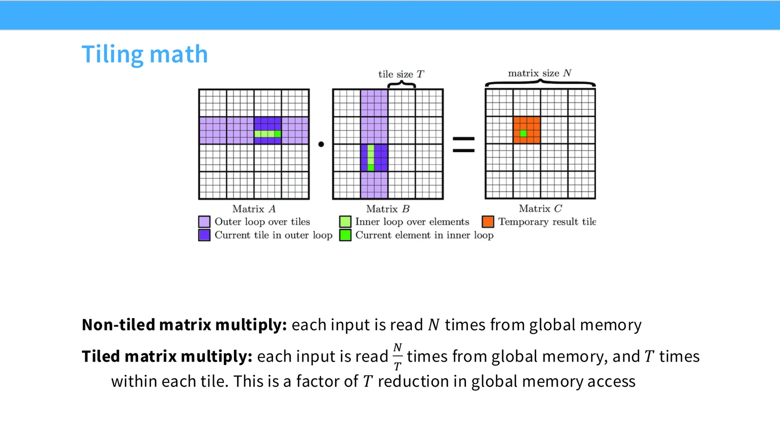
来源:CS336 Spring 2026 Lecture 5 官方幻灯片。
展开说明:Non-tiled matrix multiply: each input is read \(N\) times from global memory
读图:Slide 42 应该怎么看
这页是硬件机制或性能证据页。先看数据从哪里来、在哪里复用、是否写回 HBM;再判断瓶颈是 compute、memory bandwidth、thread scheduling 还是 alignment。GPU 优化不是让公式更漂亮,而是让数据在正确层级停留更久、让 tensor cores 少等数据。
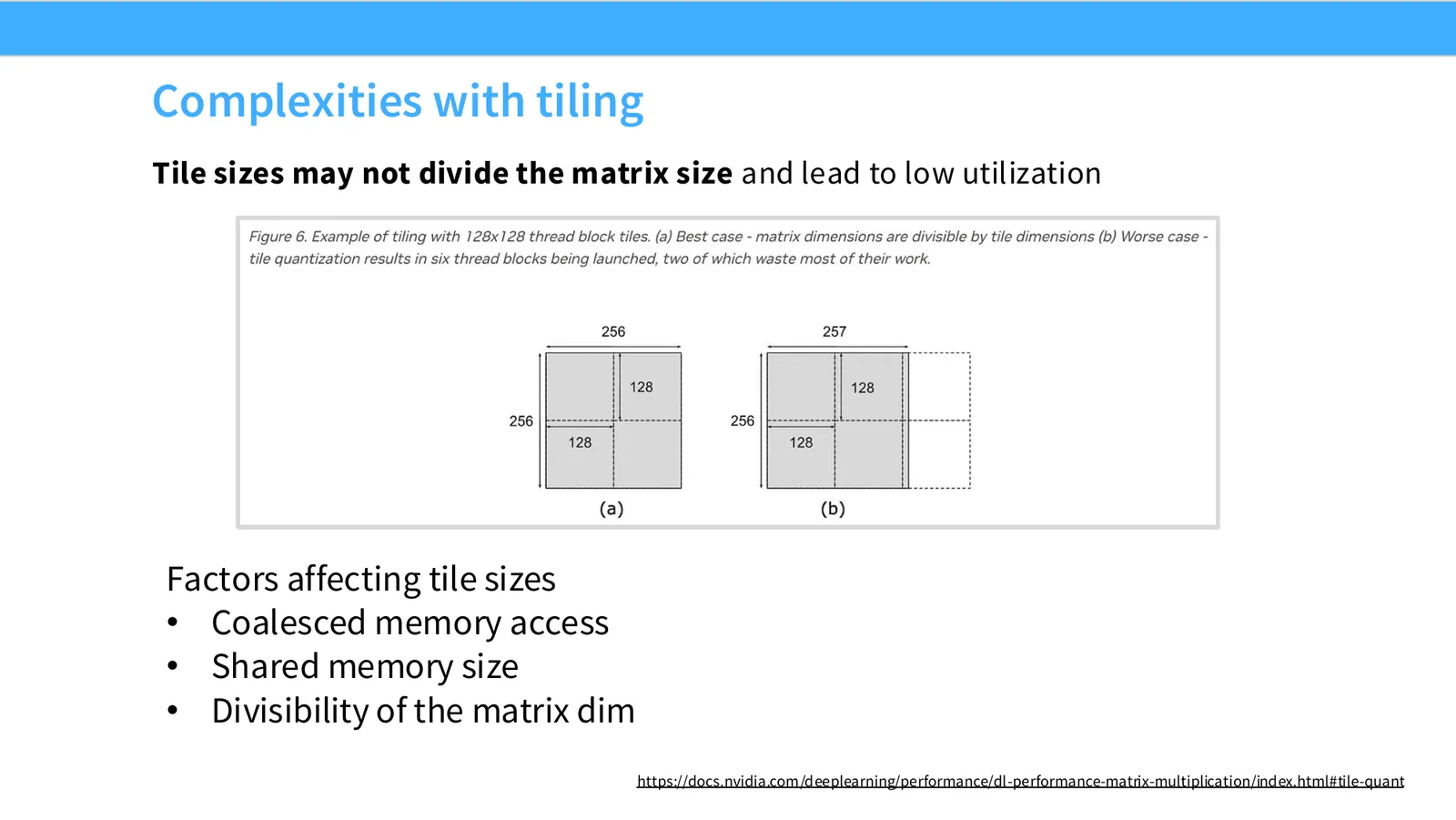
来源:CS336 Spring 2026 Lecture 5 官方幻灯片。
展开说明:Tile sizes may not divide the matrix size and lead to low utilization
读图:Slide 43 应该怎么看
这页是硬件机制或性能证据页。先看数据从哪里来、在哪里复用、是否写回 HBM;再判断瓶颈是 compute、memory bandwidth、thread scheduling 还是 alignment。GPU 优化不是让公式更漂亮,而是让数据在正确层级停留更久、让 tensor cores 少等数据。
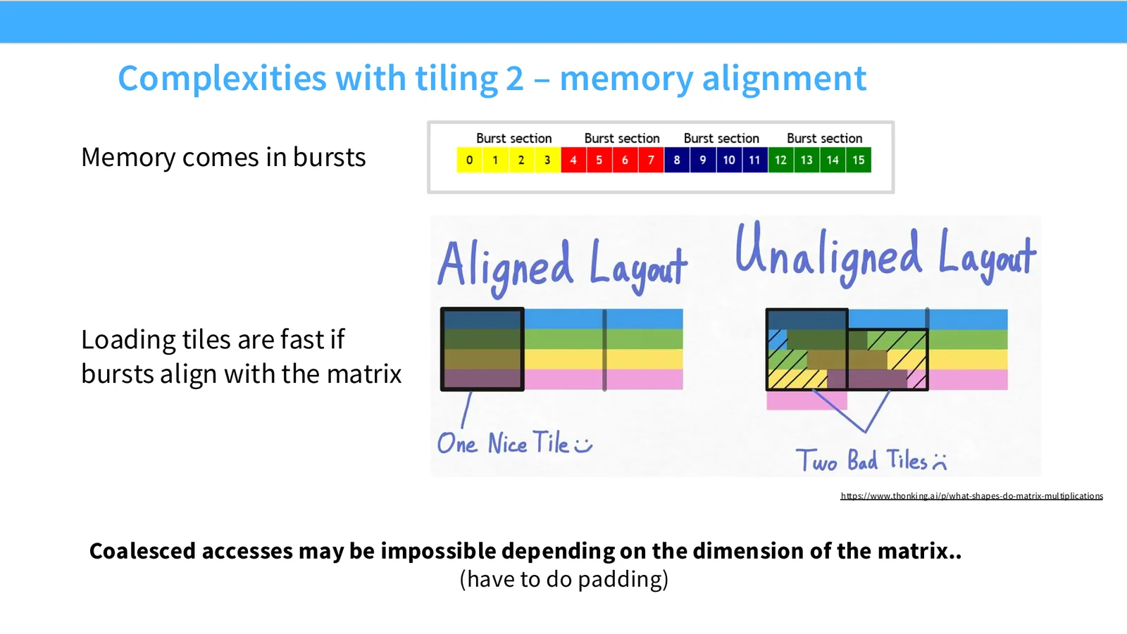
来源:CS336 Spring 2026 Lecture 5 官方幻灯片。
展开说明:Memory comes in bursts
读图:Slide 44 应该怎么看
这页是硬件机制或性能证据页。先看数据从哪里来、在哪里复用、是否写回 HBM;再判断瓶颈是 compute、memory bandwidth、thread scheduling 还是 alignment。GPU 优化不是让公式更漂亮,而是让数据在正确层级停留更久、让 tensor cores 少等数据。
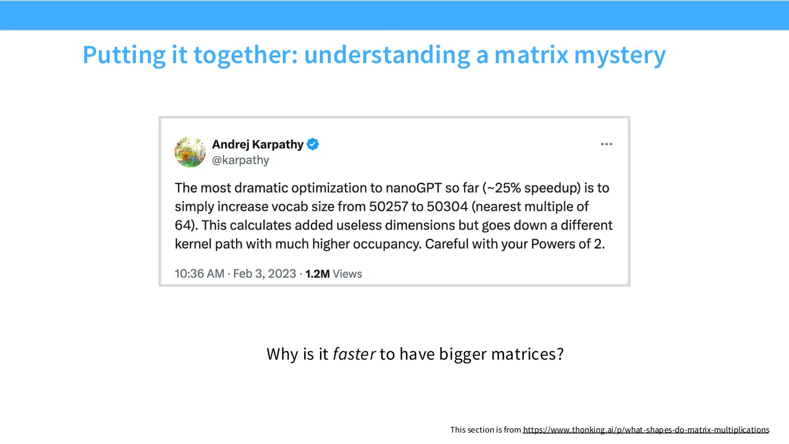
来源:CS336 Spring 2026 Lecture 5 官方幻灯片。
展开说明:Why is it faster to have bigger matrices?
读图:Slide 45 应该怎么看
这页是硬件机制或性能证据页。先看数据从哪里来、在哪里复用、是否写回 HBM;再判断瓶颈是 compute、memory bandwidth、thread scheduling 还是 alignment。GPU 优化不是让公式更漂亮,而是让数据在正确层级停留更久、让 tensor cores 少等数据。
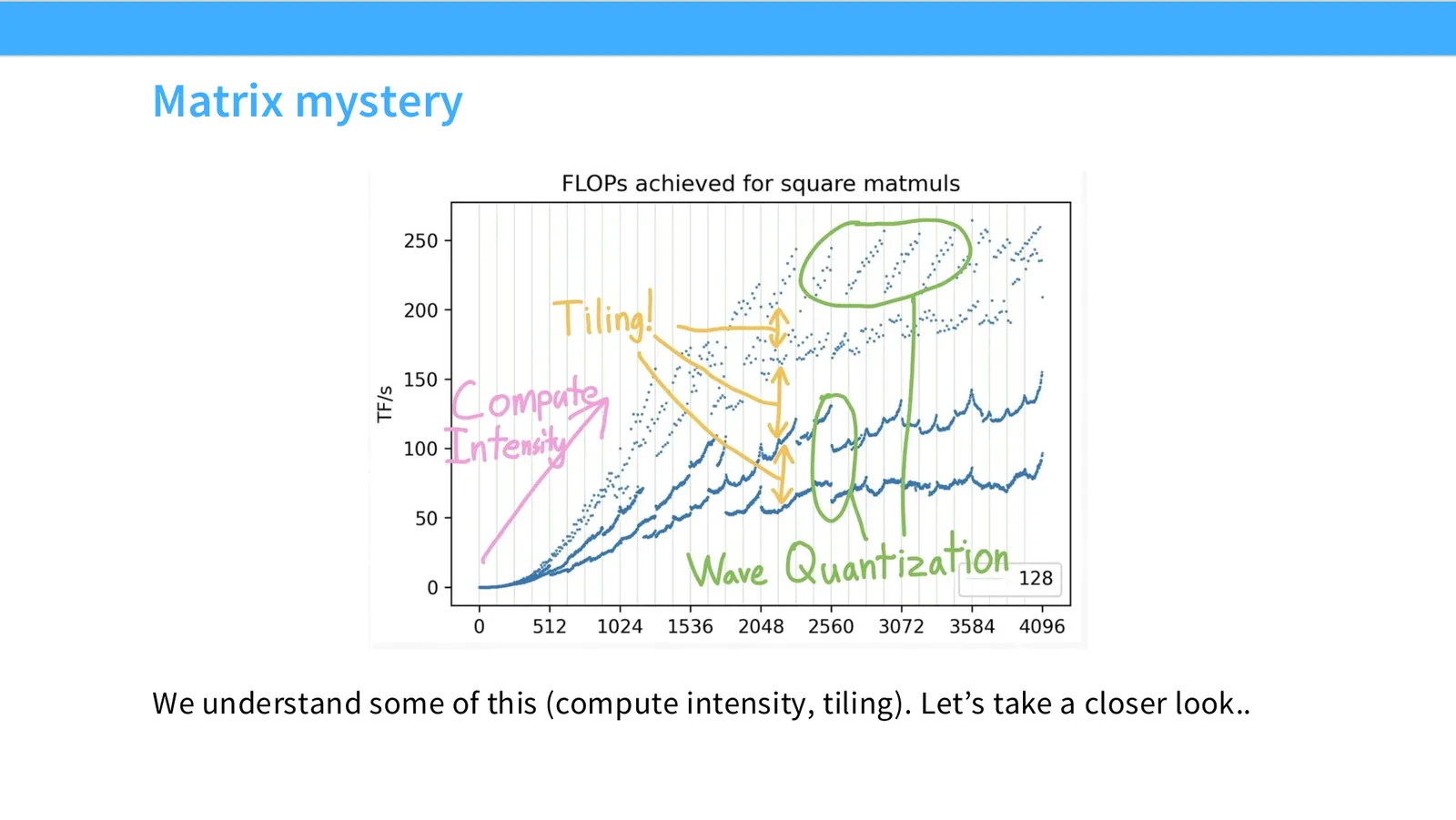
来源:CS336 Spring 2026 Lecture 5 官方幻灯片。
展开说明:We understand some of this (compute intensity, tiling). Let’s take a closer look..
读图:Slide 46 应该怎么看
这页是硬件机制或性能证据页。先看数据从哪里来、在哪里复用、是否写回 HBM;再判断瓶颈是 compute、memory bandwidth、thread scheduling 还是 alignment。GPU 优化不是让公式更漂亮,而是让数据在正确层级停留更久、让 tensor cores 少等数据。
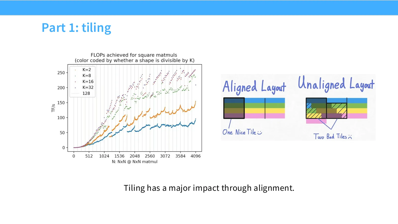
来源:CS336 Spring 2026 Lecture 5 官方幻灯片。
展开说明:Tiling has a major impact through alignment.
读图:Slide 47 应该怎么看
这页是硬件机制或性能证据页。先看数据从哪里来、在哪里复用、是否写回 HBM;再判断瓶颈是 compute、memory bandwidth、thread scheduling 还是 alignment。GPU 优化不是让公式更漂亮,而是让数据在正确层级停留更久、让 tensor cores 少等数据。
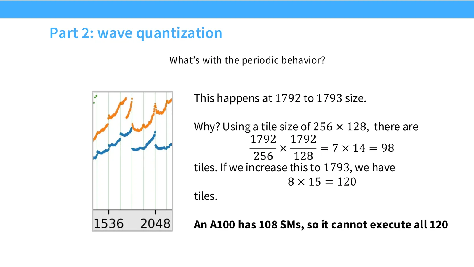
来源:CS336 Spring 2026 Lecture 5 官方幻灯片。
展开说明:What’s with the periodic behavior?
本章小结
本节的共同问题是如何减少昂贵的数据移动并提高硬件利用率。GPU 的速度来自海量并行和专用矩阵硬件,但只有当 memory access、shape、precision 和 kernel 组织匹配时,这些速度才会真正出现。
FlashAttention:把 attention 写成 IO-aware 算法
本节把前面所有硬件技巧汇总到 FlashAttention:KQV tiling、online softmax、forward pass 分块。
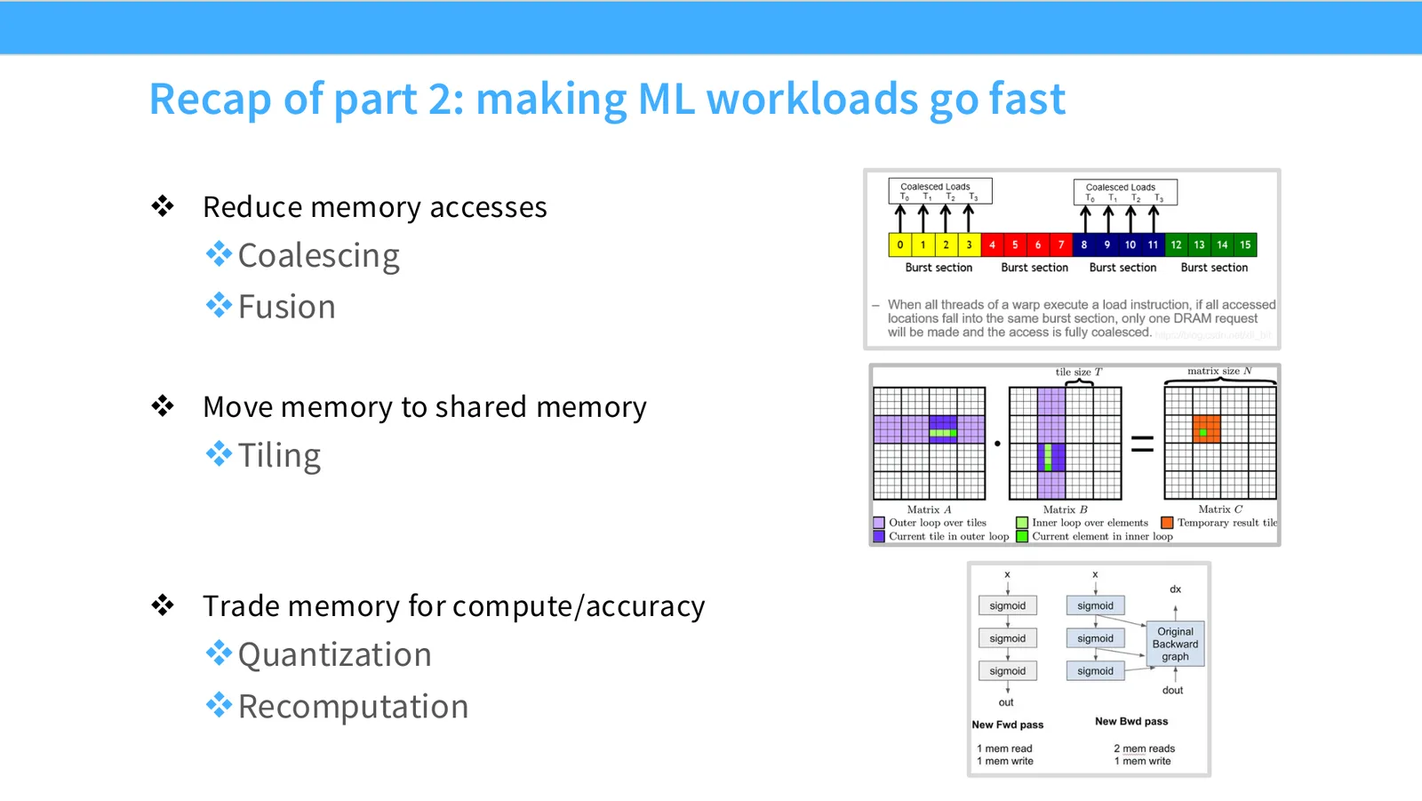
进入具体算法前,Slide 49 先总结 workload optimization 的三条主线:coalescing/fusion 减少 HBM access,tiling 把高复用数据搬到 shared memory,quantization/recomputation 则用精度或额外 compute 换 memory。FlashAttention 不是列表之外的新魔法,而是同时采用 tiling、recomputation 与 fusion,并针对 softmax 的全局归一化约束重新组织计算顺序。
来源:CS336 Spring 2026 Lecture 5 官方幻灯片。
从优化清单到算法设计
普通 kernel 优化通常保持公式和中间张量不变,只改善执行;IO-aware algorithm 会进一步问中间张量是否必须存在。Attention 的 \(QK^\top\) 分数矩阵规模为 \(n^2\),若完整写入 HBM 再读回做 softmax,即使 matmul 很快也会被 IO 限制。FlashAttention 的突破是证明 softmax 可以分块在线维护统计量,因此无需物化完整矩阵。
FlashAttention 的本质
FlashAttention 不是改变 attention 数学,而是改变计算顺序:把 Q/K/V 分块载入 SRAM,分块计算 softmax 统计量并在线更新输出,避免把完整 \(n\times n\) attention matrix 写回 HBM。
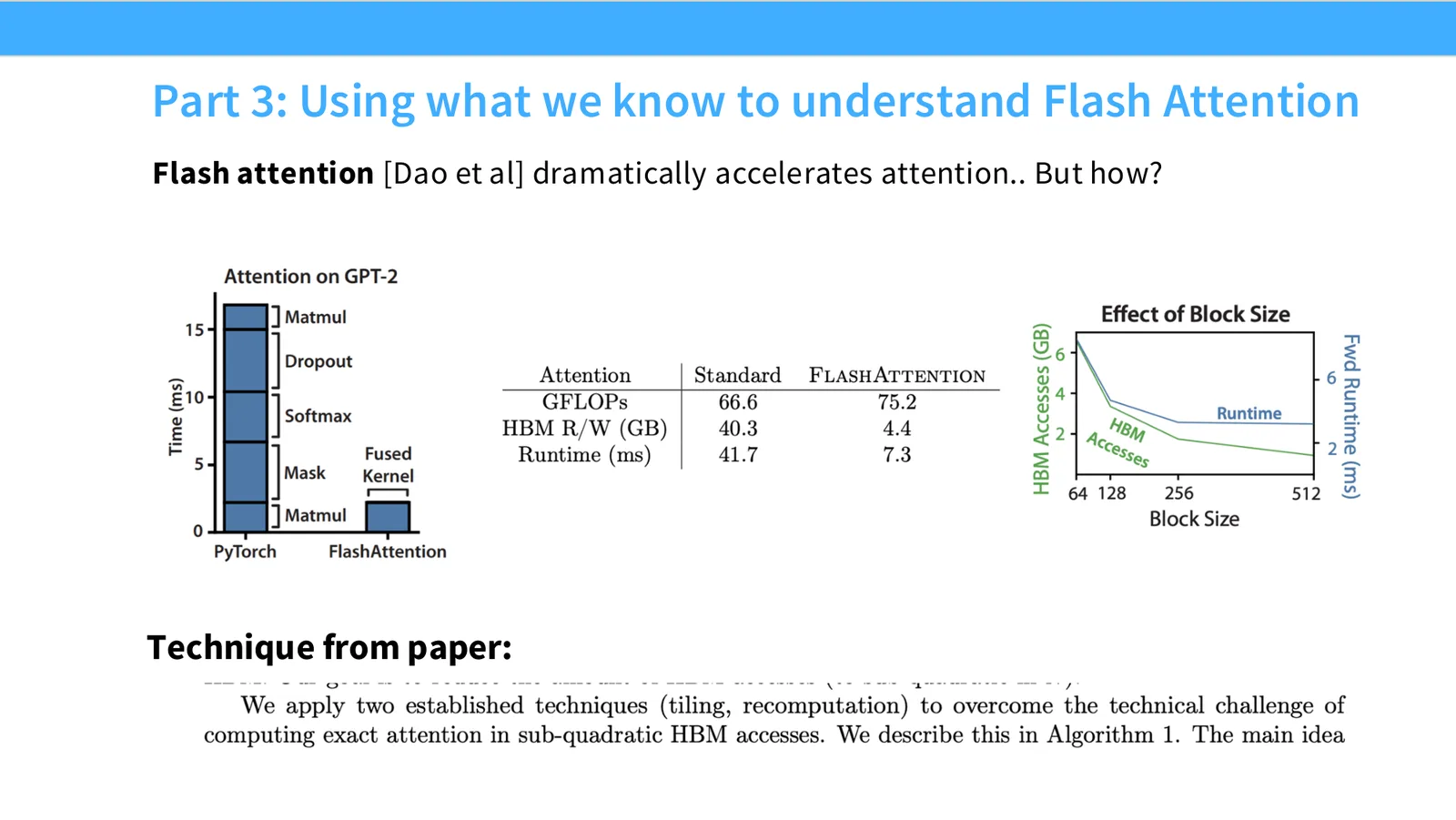
Slide 50 展示论文中的核心技术图,并提出“dramatically accelerates attention, but how?”。正确读法是先沿数据流数 HBM transactions:Q block 留在片上,K/V blocks 分批载入,每个 tile 产生局部 logits 与 partial output;在线 softmax 用 running maximum 和 normalization sum 合并不同 tiles。算法会重算部分中间值,却省下对完整 attention matrix 的写入与读取。
来源:CS336 Spring 2026 Lecture 5 官方幻灯片;Dao et al.
FlashAttention 的反直觉 tradeoff
它可能执行比 naive attention 更多的 FLOPs,因为 backward 或 tile 边界会重算 logits;但现代 GPU 的矩阵计算远快于 HBM 搬运,所以“多算、少存”反而更快。这个结论依赖硬件比例:若序列短、kernel launch 主导、片上容量不足或实现无法使用高效 tensor-core tiles,收益会缩小,必须以目标 shape 的 benchmark 为准。
来源:CS336 Spring 2026 Lecture 5 官方幻灯片。
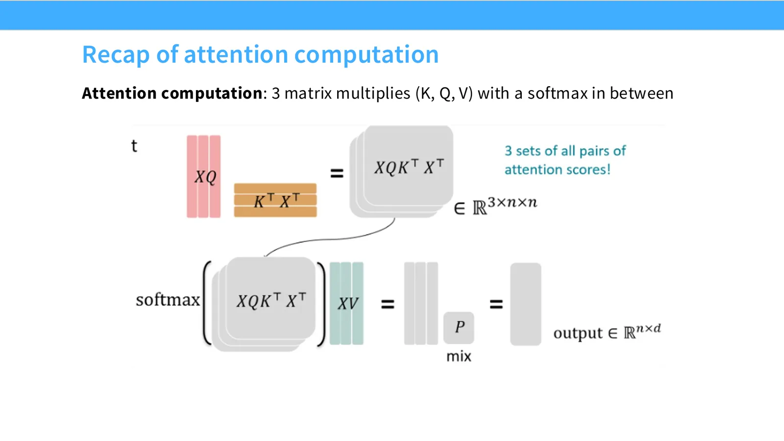
展开说明:Attention computation: 3 matrix multiplies (K, Q, V) with a softmax in between
读图:Slide 51 应该怎么看
这页是硬件机制或性能证据页。先看数据从哪里来、在哪里复用、是否写回 HBM;再判断瓶颈是 compute、memory bandwidth、thread scheduling 还是 alignment。GPU 优化不是让公式更漂亮,而是让数据在正确层级停留更久、让 tensor cores 少等数据。
来源:CS336 Spring 2026 Lecture 5 官方幻灯片。
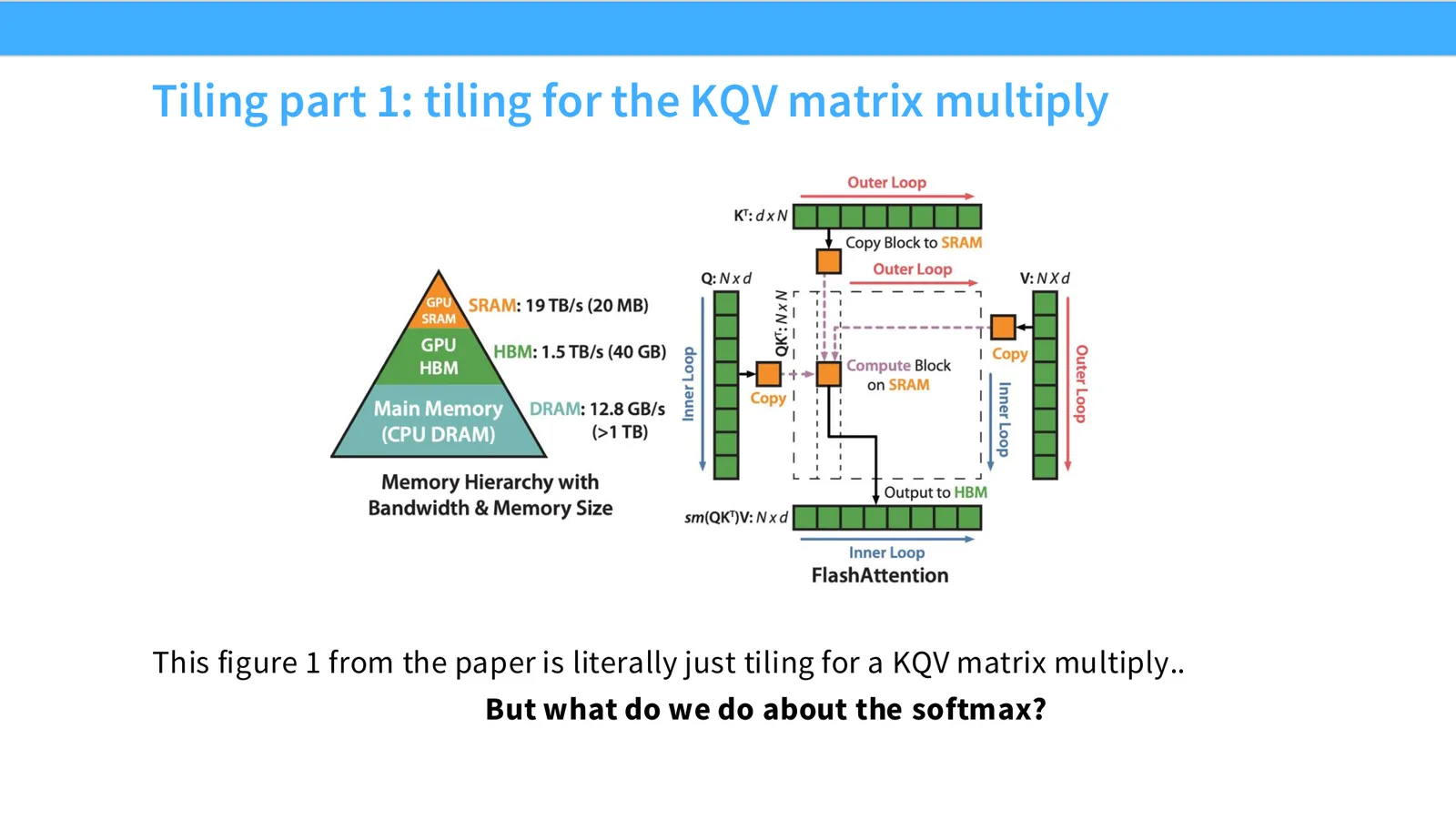
展开说明:This figure 1 from the paper is literally just tiling for a KQV matrix multiply..
读图:Slide 52 应该怎么看
这页是硬件机制或性能证据页。先看数据从哪里来、在哪里复用、是否写回 HBM;再判断瓶颈是 compute、memory bandwidth、thread scheduling 还是 alignment。GPU 优化不是让公式更漂亮,而是让数据在正确层级停留更久、让 tensor cores 少等数据。
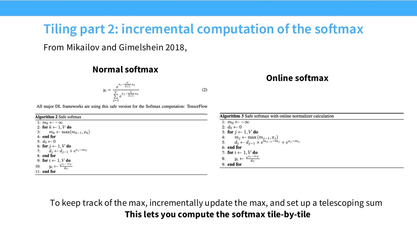
来源:CS336 Spring 2026 Lecture 5 官方幻灯片。
展开说明:From Mikailov and Gimelshein 2018,
读图:Slide 53 应该怎么看
这页是硬件机制或性能证据页。先看数据从哪里来、在哪里复用、是否写回 HBM;再判断瓶颈是 compute、memory bandwidth、thread scheduling 还是 alignment。GPU 优化不是让公式更漂亮,而是让数据在正确层级停留更久、让 tensor cores 少等数据。
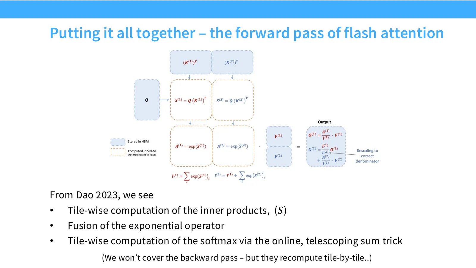
来源:CS336 Spring 2026 Lecture 5 官方幻灯片。
展开说明:From Dao 2023, we see
本章小结
本节的共同问题是如何减少昂贵的数据移动并提高硬件利用率。GPU 的速度来自海量并行和专用矩阵硬件,但只有当 memory access、shape、precision 和 kernel 组织匹配时,这些速度才会真正出现。
GPU 性能实验应该记录什么
现在 55 张源 slide 都已纳入,最后把性能故事转成实验协议。对任意 kernel 或 IO-aware algorithm,至少需要记录输入 shape、dtype、warmup/重复次数、kernel time、端到端 time、读写 byte、实现选择和硬件型号;否则 benchmark 无法复现。若比较低精度,还要报告收敛或误差;若比较 fusion/recomputation,则要报告 peak memory;若比较 tiling/FlashAttention,则要覆盖多个 sequence length、head dimension 与 batch size,而不是只展示最好点。
| 问题 | 最低证据 | 常见误判 |
|---|---|---|
| Compute-bound 还是 memory-bound? | Roofline 位置、achieved FLOP/s、effective bandwidth。 | 峰值 FLOP/s 很高就认为 kernel 应该快。 |
| 低精度是否有效? | 吞吐、转换开销、scale metadata、loss/误差曲线。 | 只按 bit 数推算 2 倍或 4 倍加速。 |
| Fusion 或重算是否值得? | kernel 数、HBM byte、peak memory、额外 FLOPs。 | 局部 kernel 更快但端到端无变化。 |
| Tiling 是否匹配硬件? | Tile shape、occupancy、shared memory、wave 数与对齐。 | 只用理论 arithmetic intensity 解释锯齿。 |
| FlashAttention 是否更快? | 目标 batch/heads/length 下 latency、memory、numerical delta。 | 只引用论文总加速,不测自己的 shape。 |
最小复现实验:从 naive attention 到 IO-aware attention
实现或调用一个会物化 \(n\times n\) scores 的 attention baseline,再与 FlashAttention kernel 比较。固定 dtype 和输出容差,扫描 sequence length、head dimension 与 batch size;记录 forward/backward time、peak memory 和数值误差。随后加入一个未参与选择 tile/kernel 的 hold-out shape。若加速只出现在对齐良好的少数维度,结论应写成“特定 shape 的 kernel 优势”,而不是笼统写成 FlashAttention 永远更快。
总结
前面已经从硬件层级一路推到 FlashAttention,现在综合这些低层细节如何支撑模型 scaling。共同规律是:低精度减少每个元素的 byte,fusion 与 recomputation 减少中间状态写回,coalescing 与 tiling 提高局部复用,而 IO-aware 算法从公式层面避免生成不必要的大矩阵。
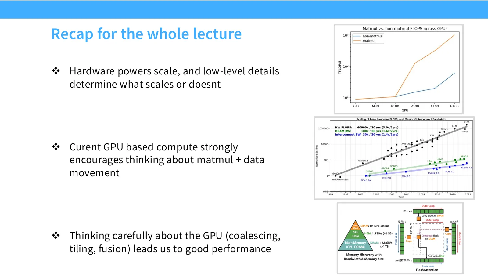
来源:CS336 Spring 2026 Lecture 5 官方幻灯片。
展开说明: Hardware powers scale, and low-level details
本章小结
本节的共同问题是如何减少昂贵的数据移动并提高硬件利用率。GPU 的速度来自海量并行和专用矩阵硬件,但只有当 memory access、shape、precision 和 kernel 组织匹配时,这些速度才会真正出现。
总结与延伸
Lecture 5 把 GPU 性能拆成三个层级:硬件结构、算子组织、算法重排。硬件层给出 SM/warp/shared memory/HBM/tensor cores;算子层使用 low precision、fusion、coalescing、tiling;算法层用 FlashAttention 这类 IO-aware 设计避免不必要 HBM 写回。
最终 takeaway
大模型训练不是“把 PyTorch 放到 GPU 上”这么简单。真正的 GPU-aware thinking 是:每个 byte 从 HBM 进来后要被复用多少次?中间结果是否必须写回?thread/warp/block 是否对齐硬件?算法能否重排成更少 IO 的形式?
拓展阅读
- NVIDIA CUDA Programming Guide and H100/B200 architecture material.
- JAX Scaling Book roofline and inference chapters.
- Dao et al. FlashAttention papers.
- NVIDIA Transformer Engine low precision documentation.