Lecture 10:GLOM——固定神经网络如何表示动态 Part-Whole Hierarchy
来源审计与证据边界:先说明 GLOM 还没有“成功”
这节课最容易被写坏的地方,不是公式,而是证据等级。Geoffrey Hinton 介绍的 GLOM 不是一个已经完成训练、在标准数据集上取得分数的模型;它首先是一份关于表示方式的设计文档:如果神经网络不能像程序一样动态申请一块内存来存 parse-tree node,那么能否用固定硬件中的动态 activity pattern 表示每张图像都不同的层次结构?本讲的价值在于把 capsule、contrastive learning、attention、distillation 与 neural field 放进一个统一假说,而不是给出已验证的产品配方。
来源:Stanford Online 官方视频 00:00:26–00:01:07。
最重要的历史边界:这是 design sketch,不是 benchmark result
Hinton 在开场直接把完整系统称为 imaginary system 和“vaporware”。原论文 arXiv:2102.12627 共 44 页,公开记录只有 2021-02-25 的一个版本。课堂提到少量 toy fragments,但没有报告端到端 GLOM 在 segmentation、recognition 或 reasoning benchmark 上的完整结果。因此下文所有“应该形成 islands”“可以用 consensus 训练”等句子都表示设计机制与可检验假设,而不是已经证明的事实。
课堂提示
讲者说自己本来在写一个系统设计文档,最后发现设计文档本身已经足够有趣;“little bits”可能存在,但整套东西不存在。保留这句自我限制非常关键,因为它决定我们应该用 architecture review 的方式阅读,而不是用 leaderboard review 的方式阅读。
三类已有思想,压成一个表示问题
GLOM 的路线不是发明一个全新的 layer,而是重新组合三个方向:Transformer 提供基于相似度的交互;unsupervised/contrastive representation learning 提供“哪些 activity 应当一致”的学习信号;neural field 提供“同一个高层对象如何在不同坐标位置生成不同低层部件”的位置条件函数。Capsule、distillation 和 recurrent settling 则贯穿其间。
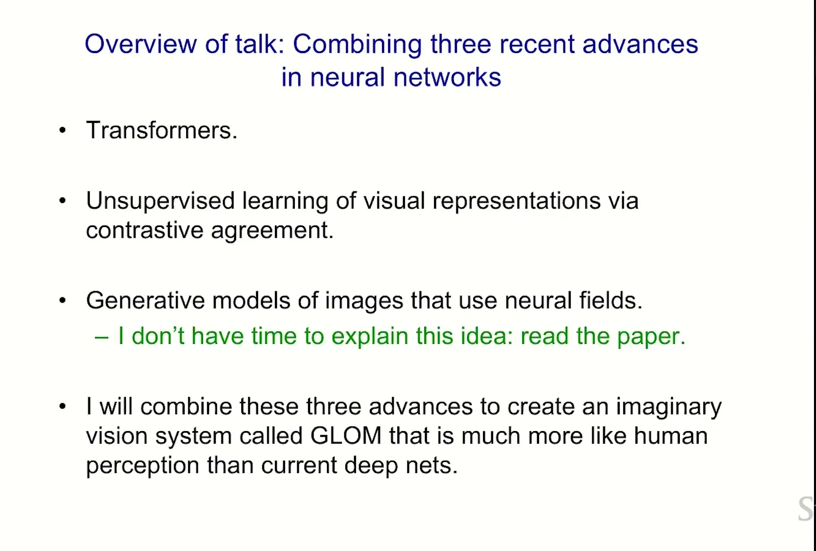
来源:Stanford Online 官方视频 00:01:08–00:01:51。
本讲使用的证据类型
| 证据类型 | 本讲能提供什么 | 不能直接推出什么 |
|---|---|---|
| 表示论动机 | 固定连接与动态 parse structure 的矛盾 | GLOM 一定可训练、一定优于现有模型 |
| 心理演示 | 人类会选择 intrinsic coordinate frame 与 alternative parse | 大脑必然实现 GLOM 的具体向量更新式 |
| 架构草图 | column、level、attention、top-down/bottom-up 的信息流 | 稳定收敛、样本效率、算力成本的实测数字 |
| 与已有论文类比 | SimCLR、BERT、Hough、NeRF 提供可复用 mechanism | 这些系统的成功会自动转移到 GLOM |
工程与脑科学不是同一个验收标准
Hinton 把神经网络研究分成两类目标:工程目标只问系统能否工作,脑科学目标还问这种机制是否可能解释 biological intelligence。共享权重、百层 ResNet 对工程师完全合理,但未必是脑的直接模型。GLOM 故意同时触碰两类问题,因此讲义必须把 engineering plausibility 与 biological plausibility 分开。
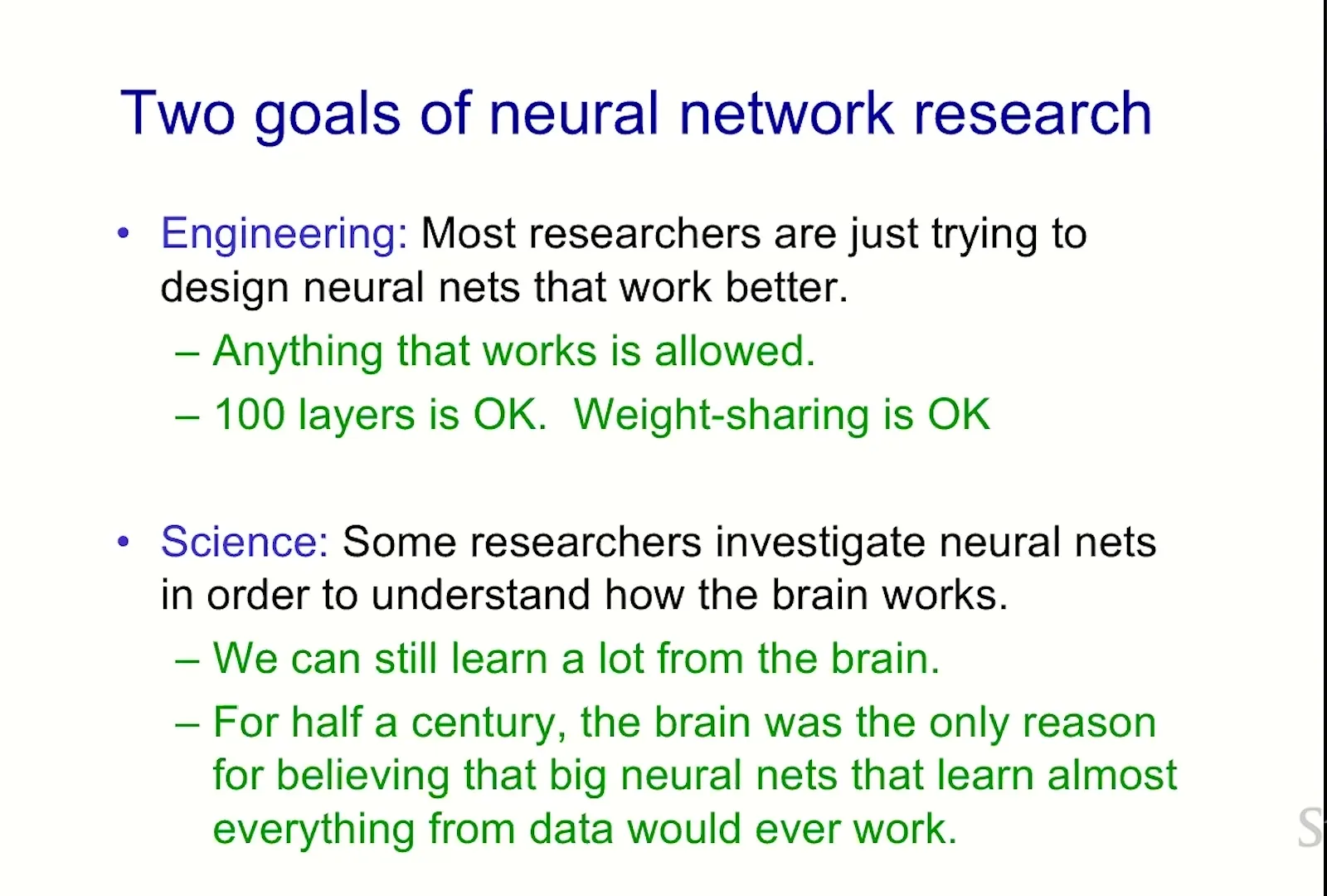
来源:Stanford Online 官方视频 00:01:52–00:02:37。
课堂提示
讲者提醒:神经网络研究曾经长期依赖一个朴素信念继续存在——大脑已经证明复杂学习在原则上可能。这个历史判断不是说工程模型必须复制大脑,而是说 biological existence proof 仍可启发新的 representation question。
本章小结
本讲讨论的是一个历史上明确受限的设计提案。阅读顺序应是:先理解它要解决的 representational contradiction,再检查每个机制是否形成可计算、可训练、可证伪的假说,最后才讨论它与现代 object-centric model 或 world model 的关系。
固定硬件与动态 Parse Tree 的矛盾
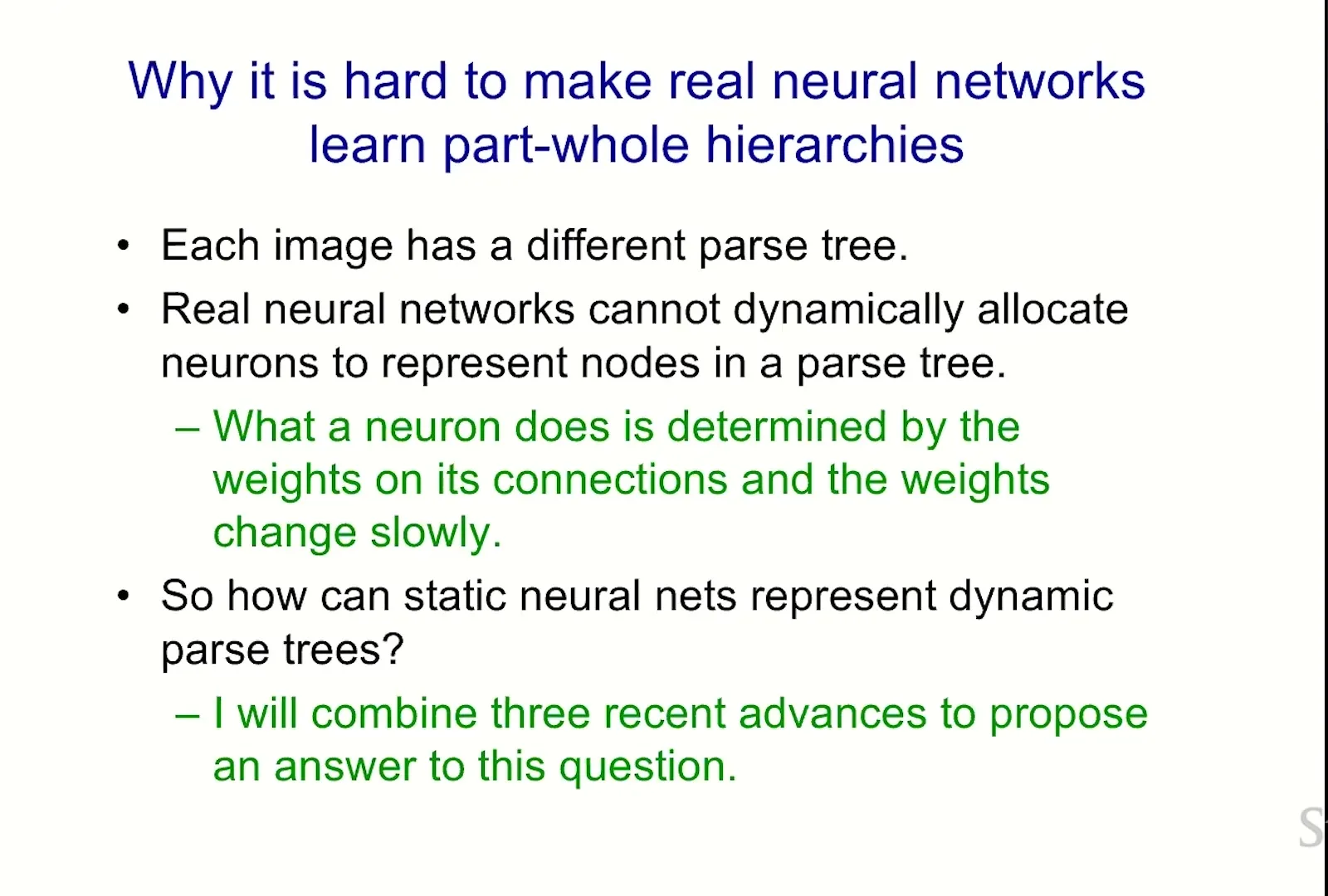
一张图像中的“眼睛属于脸、轮子属于车”并不是固定树;换一张图,节点数、部件种类和连接方式都会改变。程序可以动态申请内存并写 pointer,真实神经元却不能在几毫秒内重写全部连接权重。GLOM 的核心问题因此可以写成:在不动态分配 neuron identity 的条件下,怎样让 activity 表示一个每次输入都变化的 parse tree?
来源:Stanford Online 官方视频 00:02:38–00:04:13。
核心矛盾
网络连接参数 \(\theta\) 在样本之间变化很慢,而输入 \(I\) 对应的结构 \(\mathcal T(I)\) 每次都不同。目标不是让 \(\theta\) 直接存一棵固定树,而是让由 \(\theta\) 计算出的动态状态 \(\mathbf E(I)\) 在一次 inference 内编码 \(\mathcal T(I)\)。
Symbolic allocation、Capsule routing 与 universal capsule
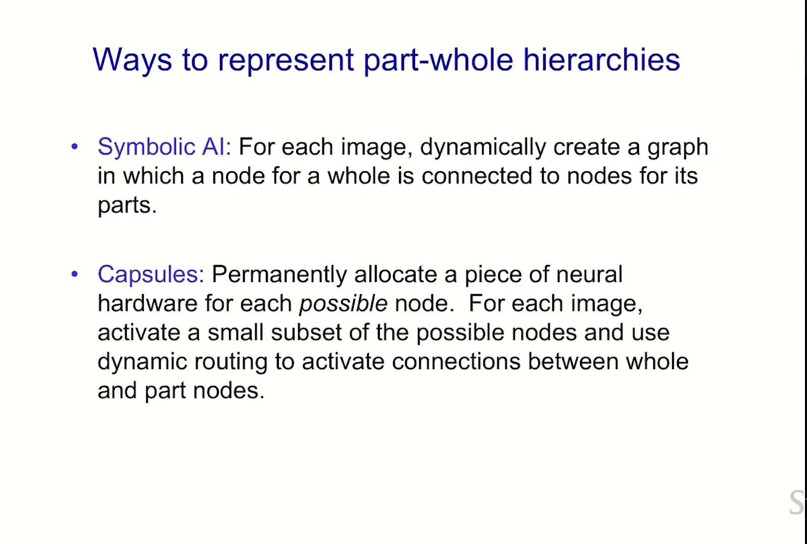
Symbolic AI 的答案很直接:拿一块 memory 当 node,再写入指向其他 node 的 pointer。早期 capsule 路线则预先分配许多可能节点,每个 capsule 专门表示一种 entity;一次输入只激活其中少量 capsule,并用 routing 决定 parent-child connection。这避免了动态创建 neuron,却带来大量静默硬件、type-specific capsule 与 routing optimization。
来源:Stanford Online 官方视频 00:04:14–00:05:35。
课堂提示
Hinton 用一句很有教学价值的话评价研究想法:有些 idea “want to work”,有些不想工作;capsule 介于两者之间,经过大量努力可以工作,但过程艰难。这不是对 capsule 的否定,而是在提醒我们:结构先验越强,optimization contract 越必须讲清楚。
GLOM 把 capsule 改成 universal capsule:硬件仍按空间位置组织成 column,但每个 column 的同一层级 embedding 不再预先绑定“只能表示鼻子”或“只能表示轮子”。它可以表示任意 identity 与 pose;“它这次是什么”由 activity 决定,而不是由 capsule 的固定类型决定。
Column、level 与 island of agreement
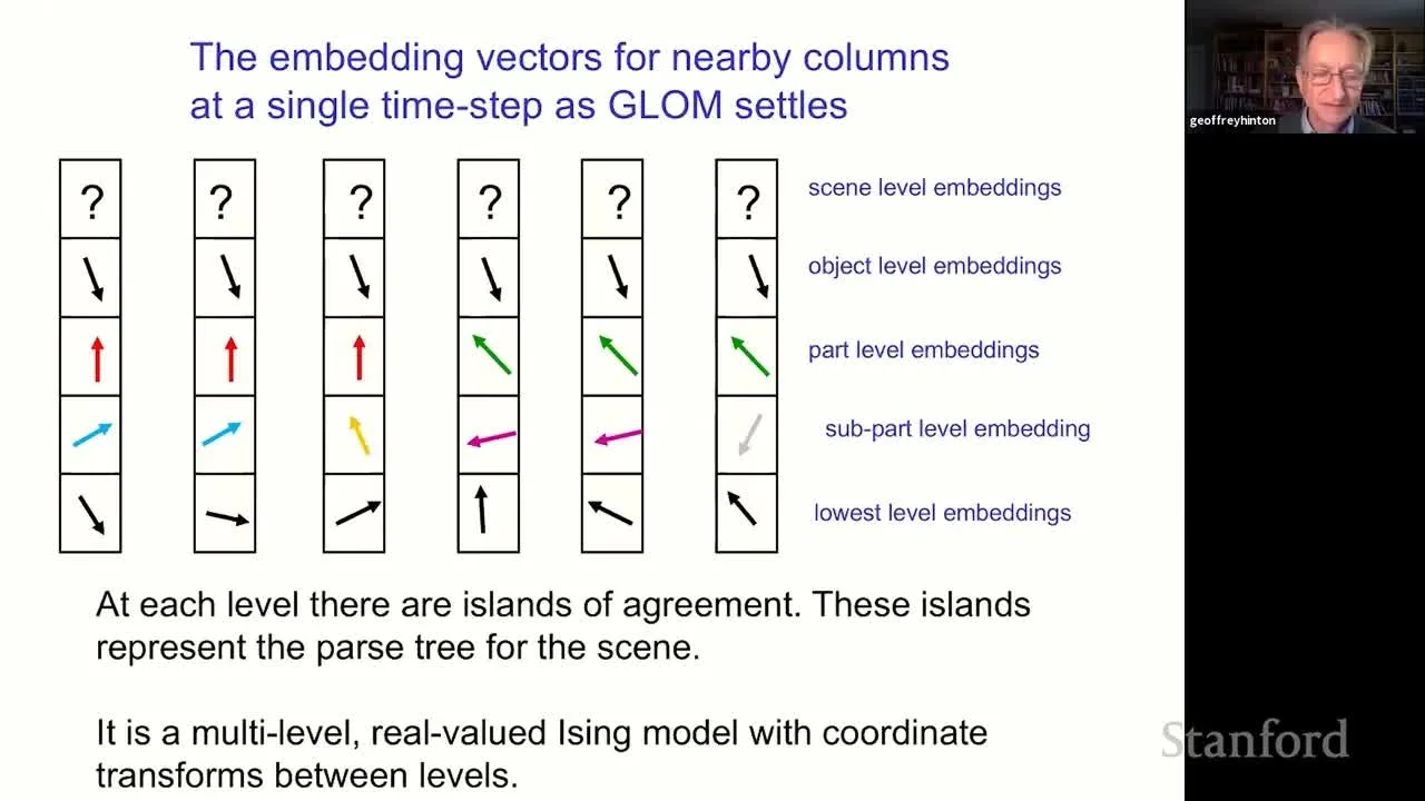
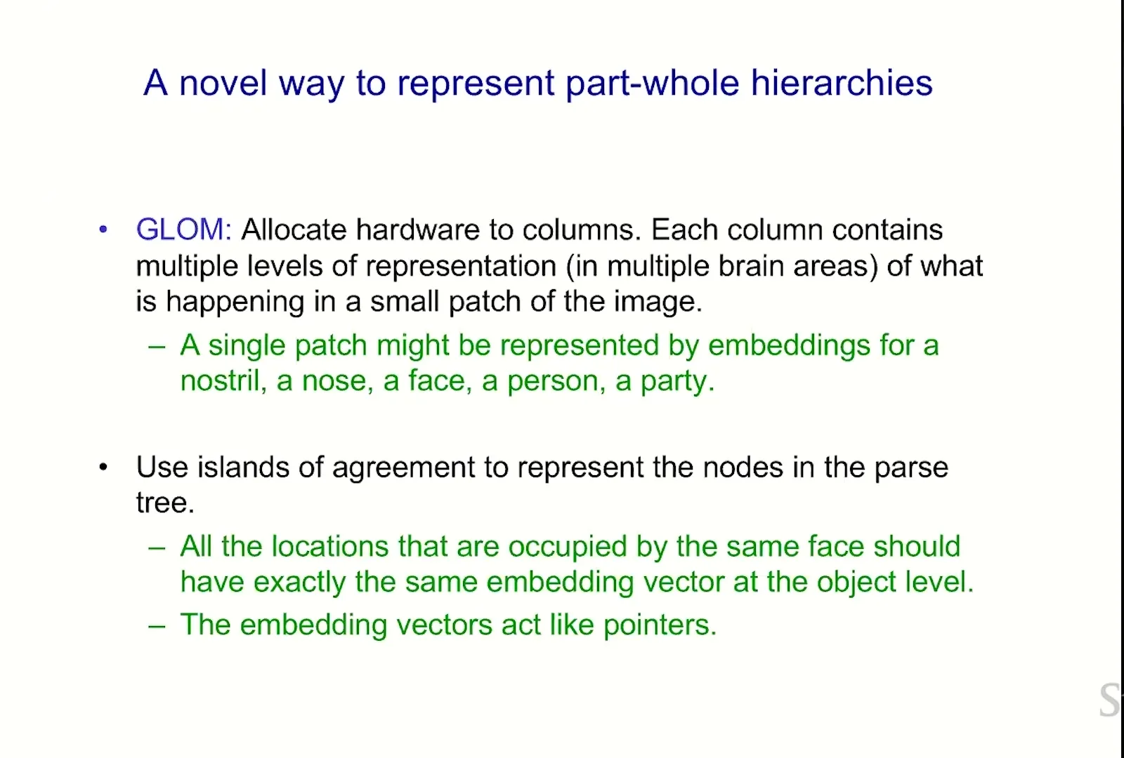
把图像划成空间位置 \(x\in\mathcal X\),每个位置建立一个 column;column 内有多个层级 \(\ell=0,1,\ldots,L\)。同一位置可能从低到高表示纹理、nostril、nose、face、person、scene。GLOM 不为“face node”分配一颗专用 neuron,而让属于同一 face 的位置在 face level 上逐渐形成近似相同的 embedding。
来源:Stanford Online 官方视频 00:05:36–00:08:29。
令 \(\mathbf e_{x,\ell}^{(t)}\in\mathbb R^d\) 表示位置 \(x\)、层级 \(\ell\)、settling step \(t\) 的动态向量。一个候选 island \(S\) 可用下面的近似条件描述:
其中,\(S\) 是某个层级上的位置集合,\(d\) 是 embedding 维度,\(t\) 是 recurrent inference 的迭代步,\(\varepsilon\) 是“足够相似”的容差。课堂二维箭头只用方向表示 equality;它不是说真实表示只有两个维度,也不是要求所有分量严格 bitwise identical。
动态 activity 才是 pointer
参数权重决定“如何更新向量”,embedding activity 决定“当前输入里这个位置属于谁”。因为 activity 每张图都能变化,固定网络可以形成不同 islands;这些 islands 及其跨层对应关系承担了 dynamic parse-tree node 的角色。
来源:Stanford Online 官方视频 00:08:30–00:09:15。
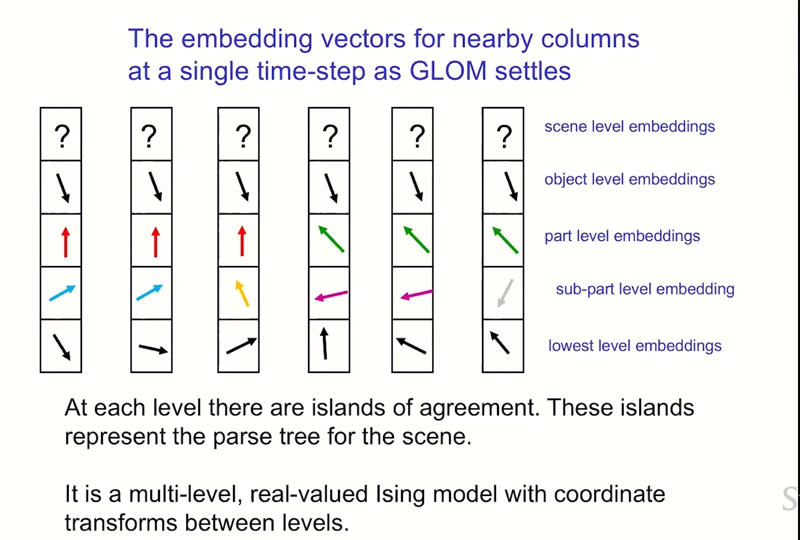
读图:箭头方向只编码“是否相同”
先沿横轴看空间位置,再沿竖轴看抽象层级。最底层黑色箭头各不相同,表示每个 patch 的局部内容不同;向上后,连续位置出现同方向红、绿、蓝箭头,表示它们在该层被解释为同一 part、object 或 scene。问号表示尚未 settle 的状态。图不提供 embedding 的真实数值、置信度或边界阈值,因此只能读出设计意图,不能读成 segmentation result。
术语消化:不要把四个对象混成一个词
| 术语 | 在 GLOM 中是什么 | 容易混淆之处 |
|---|---|---|
| column | 一个空间位置上的多层硬件与状态 | 不是 CNN channel,也不是数据库 column |
| level | part-whole hierarchy 的一个抽象尺度 | 不是普通深层网络的第 \(k\) 层同义词 |
| embedding | 某位置、层级、时间步的动态 activity vector | 不是固定词向量,也不是网络权重 |
| island | 同层相邻或可关联位置形成的近似一致区域 | 不是输入中预先给出的 mask,也不保证等于 ground-truth object |
比普通空间分割更宽的结构
Hinton 特别指出,island 不必只表达连续图像区域。在语言中,短语的两个 fragment 可以在更高层获得相同表示,即使它们在序列中并非一个连续二维块。这意味着 GLOM 想表达的是“共同属于一个 higher-level entity”,而不只是 connected-component segmentation。
课堂提示
课堂用 “shut” 与 “up” 举例:低层是两个不同 fragment,高层可以共享 “shut up” 的向量。这个例子提示我们,island 的拓扑由 neighborhood 与 attention graph 决定,不应被狭义理解为像素平面上的实心色块。
Island 不自动等于 object
即使某层出现大块相似向量,也可能来自 texture、背景、错误 collapse 或 optimization shortcut。若要声称“模型发现对象”,还需 segmentation alignment、intervention、cross-view consistency 与下游因果使用等证据。本讲没有提供这些实验。
本章小结
GLOM 用 universal capsule 与 dynamic embeddings 替代 type-specific node allocation。它的关键主张不是“多做几层 attention”,而是让每个层级的 agreement pattern 本身成为 parse structure;真正困难的下一步,是让这种 agreement 既能形成又不会全局塌缩。
坐标系为何是 Part-Whole Relation 的核心
如果一个 nostril 支持“这里有一个 nose”,它不仅要预测 identity,还要预测 nose 的 position、orientation 与 scale。换句话说,part-whole relation 不是一个离散标签,而是 intrinsic coordinate frame 之间的变换。Hinton 用一组心理实验先让听众感受到:我们对同一组线条的理解,会随内部 reference frame 改变。
来源:Stanford Online 官方视频 00:09:16–00:13:31。
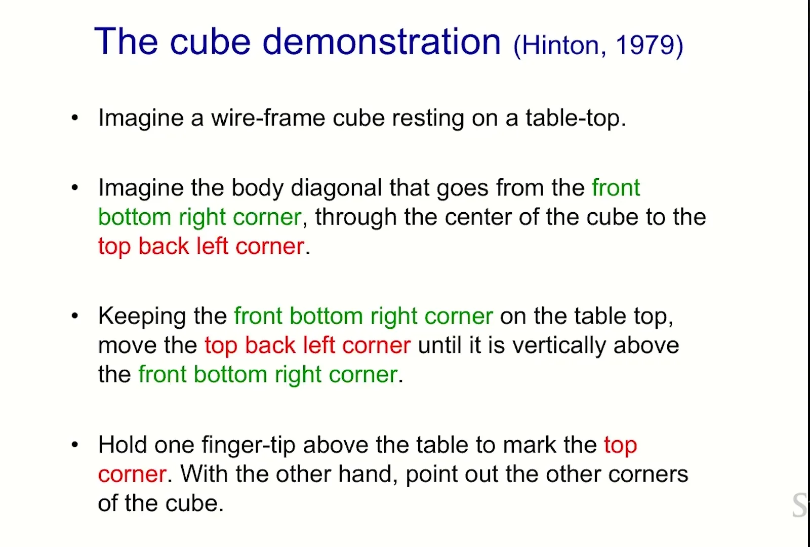
Cube demonstration:难点不是旋转,而是换 frame
课堂要求听众想象一个 wire-frame cube,把原来的 body diagonal 旋转到竖直方向,再指出其他角的位置。许多人并不是不会三维几何,而是习惯把 cube 放在“桌面水平、竖直边朝上”的 intrinsic frame 中;一旦强制使用陌生 frame,同一对象的 internal representation 会剧烈改变。
来源:Stanford Online 官方视频 00:13:32–00:16:07。
读图:任务真正改变的是 intrinsic frame
先找原来接触桌面的 front-bottom-right corner,再找与它相对的 top-back-left corner;课堂要求把这条 body diagonal 旋成竖直轴。其他六个 corner 的几何关系没有消失,但熟悉的“底面水平、竖边朝上”坐标系被撤走。若听众难以定位角点,证据支持的是 reference-frame dependence,而不是一般三维旋转能力不足。
心理实验能证明什么
它说明人类 reasoning 会选择并依赖 reference frame,且更换 frame 会改变可访问的关系;它不能证明神经元一定用 GLOM embedding、matrix capsule 或某个特定 attention rule。这里的证据角色是 motivation,不是 implementation identification。
Six rods:同一输入可以有完全不同的 parse
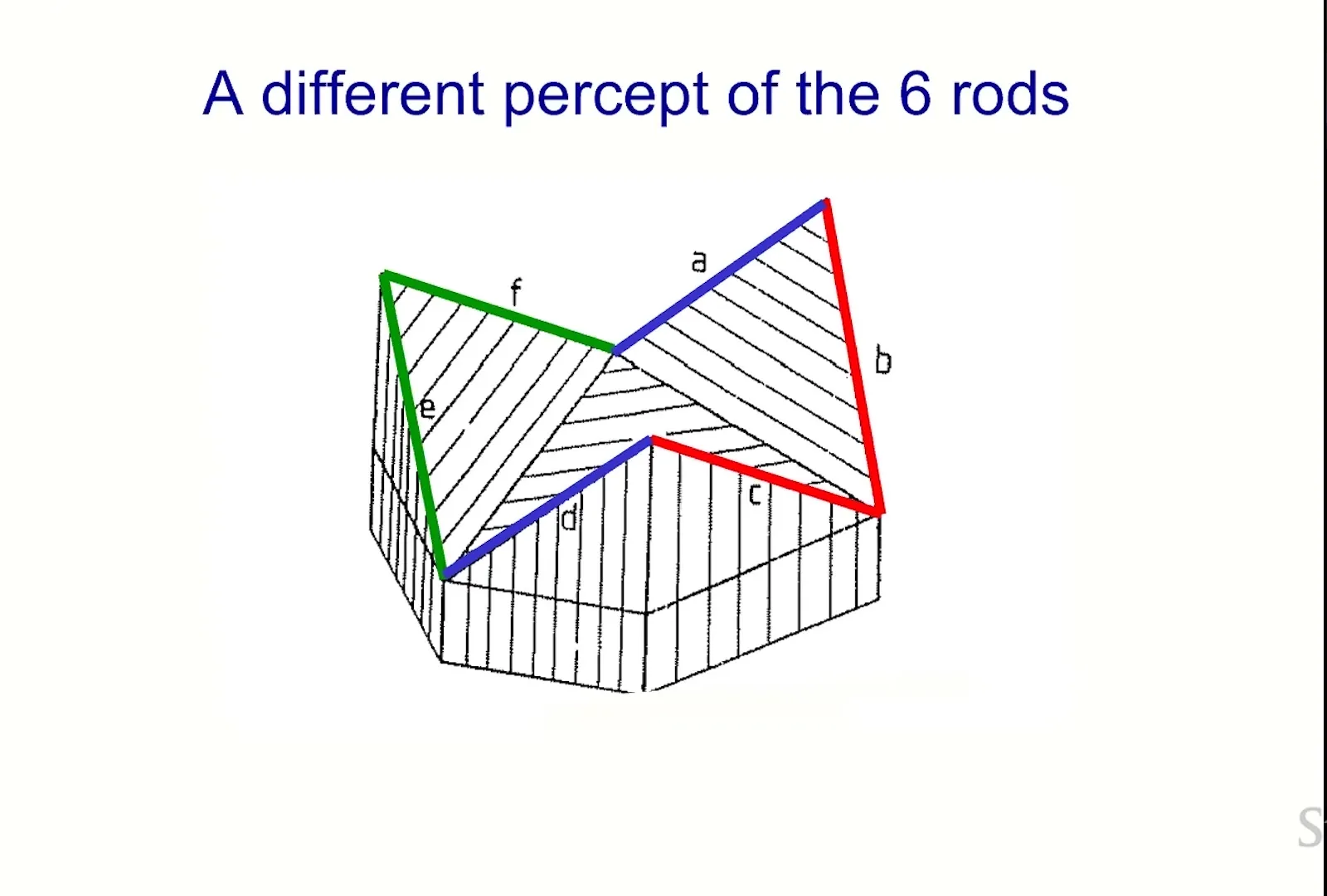
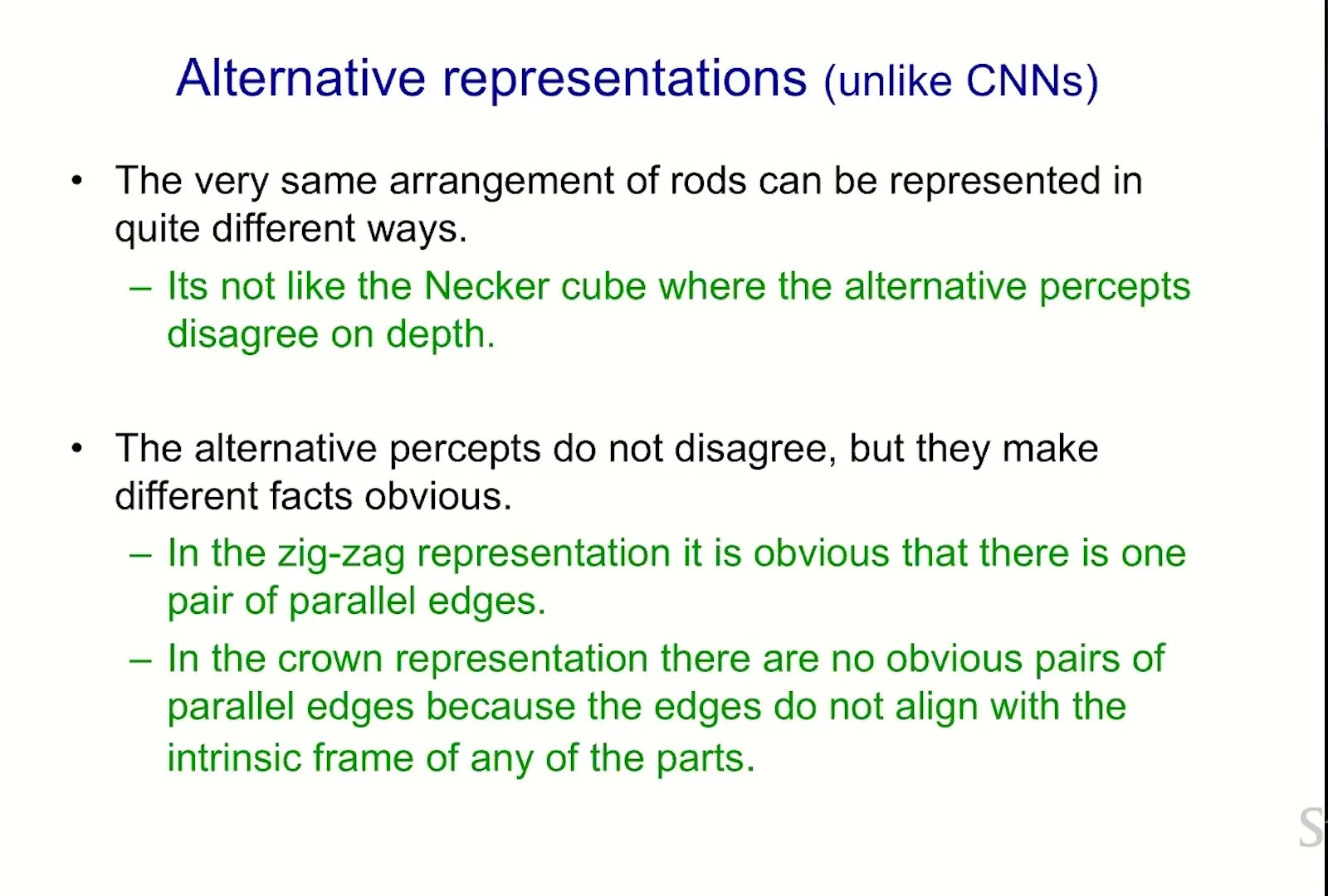
六根杆既可被看成一个三瓣 crown,也可被看成 central rectangle 加若干斜瓣。两种 percept 对外部线段位置没有争议,却让哪些边“天然成组”、哪些边显得 parallel 完全不同。Hinton 将它类比为一句话的 structural ambiguity:truth condition 可能相同,parse 却不同。
来源:Stanford Online 官方视频 00:16:08–00:16:55。
来源:Stanford Online 官方视频 00:16:56–00:17:55。
课堂提示
讲者强调这不像 Necker cube:不是你相信外部世界的 depth 改变了,而是你用另一种结构看同一事实。他用 “next weekend we should be visiting relatives” 的两种句法读法说明:representation change 不一定改变 truth condition。
Intrinsic relation 放进 weights,viewer pose 放进 activity
“crown 与 flap 的固定关系”应当随 viewpoint 保持不变,适合由 learned weights 表示;“crown 相对观察者的姿态”则随视角变化,适合由 dynamic activity 表示。课堂图中的 \(R_{wx}\)、\(R_{wv}\)、\(R_{xv}\) 可理解为在 object/part/viewer frames 之间的变换。
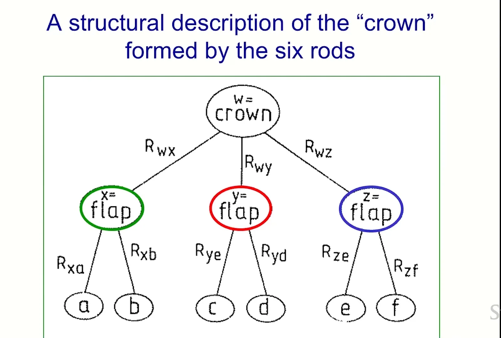
来源:Stanford Online 官方视频 00:17:56–00:17:59。
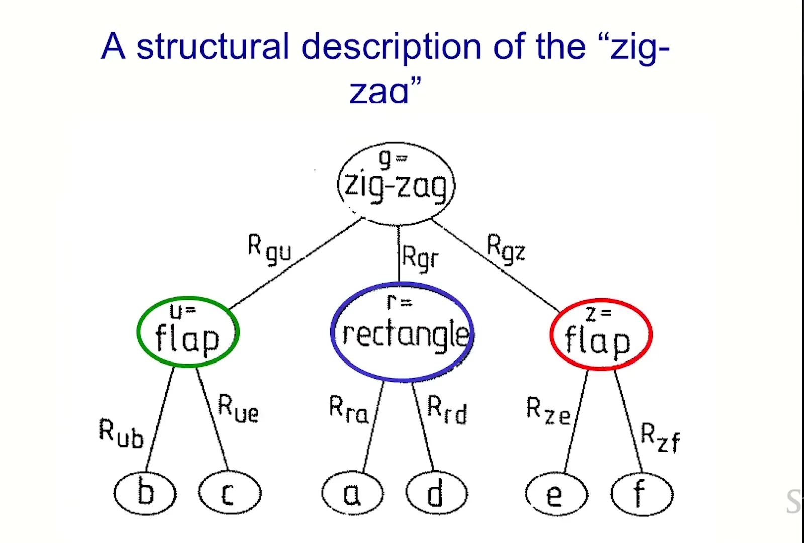
来源:Stanford Online 官方视频 00:18:00–00:20:41。
读图:比较 node grouping,而不是比较线段位置
两棵树的叶节点仍是同一组六根 rods;变化的是中间 node:crown parse 把三块 flap 组织到同一 whole,zig-zag parse 则突出 rectangle 与上下斜瓣。边上的 \(R\) 表示 intrinsic frame relation。读图时先比较哪些叶子共享 parent,再比较哪些 relation 随 viewpoint 应保持不变;不要把两张图误认为两个不同外部物体。
一种简化的 composition 可写为:
其中,\(R_{xw}\) 表示 part \(x\) 相对 whole \(w\) 的 intrinsic relation,\(R_{wv}\) 表示 whole 相对 viewer \(v\) 的当前 pose,\(R_{xv}\) 是推得的 part-to-viewer pose。不同 convention 可能改变乘法顺序;教学重点是把 viewpoint-invariant knowledge 与 viewpoint-dependent state 分开。
Matrix equation 不是课堂实现承诺
GLOM 论文讨论多种 pose/identity representation,并没有要求所有 relation 都必须是一张显式刚体变换矩阵。实际 embedding 还要容纳 identity、uncertainty、texture 与非刚体结构。把所有语义硬塞进 \(SE(3)\) 会过度简化。
Mental image 不是 pixel buffer
Hinton 的 mental imagery 观点是:内部图像可以是 structural description 加一组 viewer-relative transforms。为了回答空间问题,人会隐式选择 orientation、scale 与 position;如果换一个 frame,推理路径与“显眼关系”也会变化。
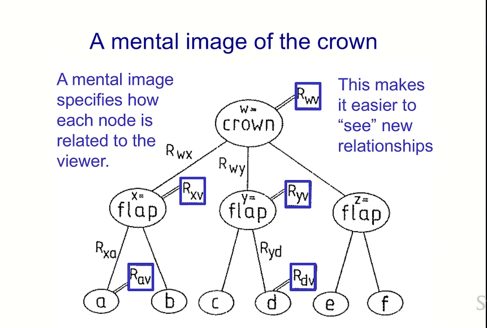
来源:Stanford Online 官方视频 00:20:42–00:22:01。
课堂提示
课堂让听众想象“向东一英里、向北一英里、再向东一英里”。多数人会默认 north 朝上、选定某个尺度与画面位置,尽管解题并不要求这些选择。这个小实验揭示:reference frame 往往是 reasoning 的隐变量。
本章小结
Part-whole hierarchy 需要同时表达 identity 与 pose。GLOM 想把稳定的 relation knowledge 放进网络函数,把输入特定的 viewpoint 与 parse 放进 embedding activity;cube、six rods 与 mental imagery 为这种分工提供认知动机,但不替代模型实验。
Contrastive Learning:Agreement 是起点,不是答案
Islands 的表面目标是“同一 entity 的不同位置得到相同向量”,这与 contrastive learning 很像。但普通 image-level objective 只知道两个 crop 来自同一张图,未必知道它们属于同一 scene、同一 object 还是不同 objects。GLOM 借用 agreement 与 anti-collapse 思想,却必须把它改造成 level-specific、local、pose-aware 的动态过程。
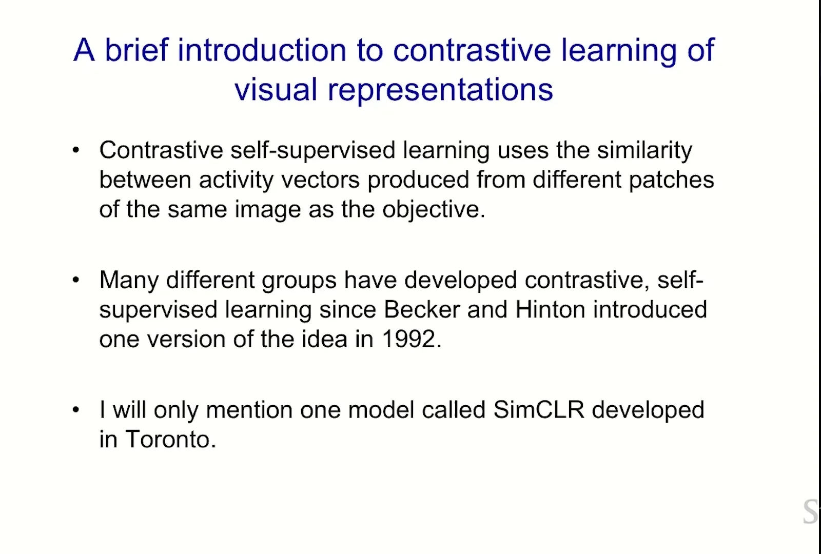
来源:Stanford Online 官方视频 00:22:02–00:24:15。
SimCLR 的正样本、增强与 collapse
上一节只说“agreement 可以学表示”,还没有说明如何避免所有向量一起相等。本节用 SimCLR 把这个缺口补齐:先明确 positive pair 的生成方式,再观察 naïve agreement 为什么 collapse,最后把这条教训带回 GLOM 的 local islands。SimCLR 对图像 \(x\) 采样两个增强视图 \(\tilde x_i,\tilde x_j\),经共享 encoder \(f\) 与 projection head \(g\) 得到 \(\mathbf z_i,\mathbf z_j\)。颜色扰动防止模型只用 color histogram 取巧;正样本应接近,不同图像的样本应至少被区分。
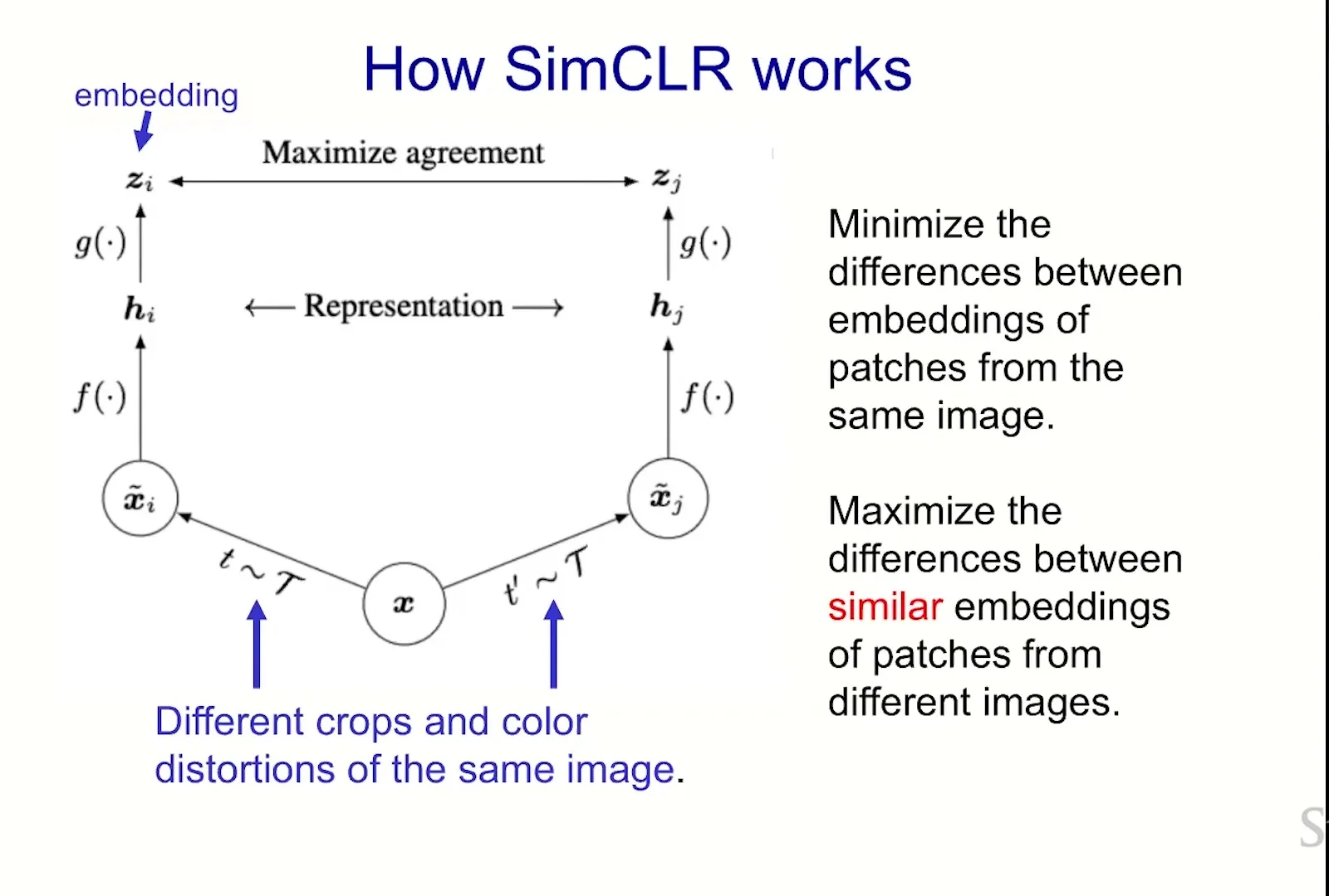
来源:Stanford Online 官方视频 00:24:16–00:25:07。
读图:先分清 \(h\) 与 \(z\)
左右两路从同一原图采样不同 crop 与颜色扰动,经共享 \(f\) 得到 representation \(h_i,h_j\),再经 projection head \(g\) 得到用于 contrastive objective 的 \(z_i,z_j\)。图中的“拉近/推远”发生在 projection space;下游 linear probe 常读 encoder representation。这个差别说明训练目标所在空间与最终使用空间可以不同,也提醒我们 GLOM 的 consensus target 必须明确作用在哪个 level 与 state。
若只最小化同图 pair 的距离,最容易的解是所有输入都映射到常量 \(\mathbf c\):
其中,\(f\) 是 encoder,\(x\) 是任意输入,\(\mathbf c\) 是统一常量表示。这会让所有 positive loss 归零,却完全没有信息。InfoNCE 一类 objective 通过同 batch negatives 或其他 anti-collapse mechanism 阻止该解。这里不展开完整温度归一化推导,重点是“agreement 必须与 separation 同时设计”。
Agreement 目标的第一风险:全局塌缩
“让相似位置更相似”不能独立存在。GLOM 需要 local neighborhood、bottom-up/top-down evidence、identity-pose prediction、level separation 与训练 objective 共同阻止整个图、所有层、所有样本变成一个向量。本讲提出了信号来源,但没有给出大规模稳定性证明。
Linear probe 只证明可线性读出
自监督训练后冻结 encoder,再训练一个线性分类器,可以测试表示是否包含容易读出的 label information。好成绩说明 feature 有用,但不说明表示已显式分解 part、whole、pose,也不说明在 generation、robustness 或 causal reasoning 上等价于 supervised model。
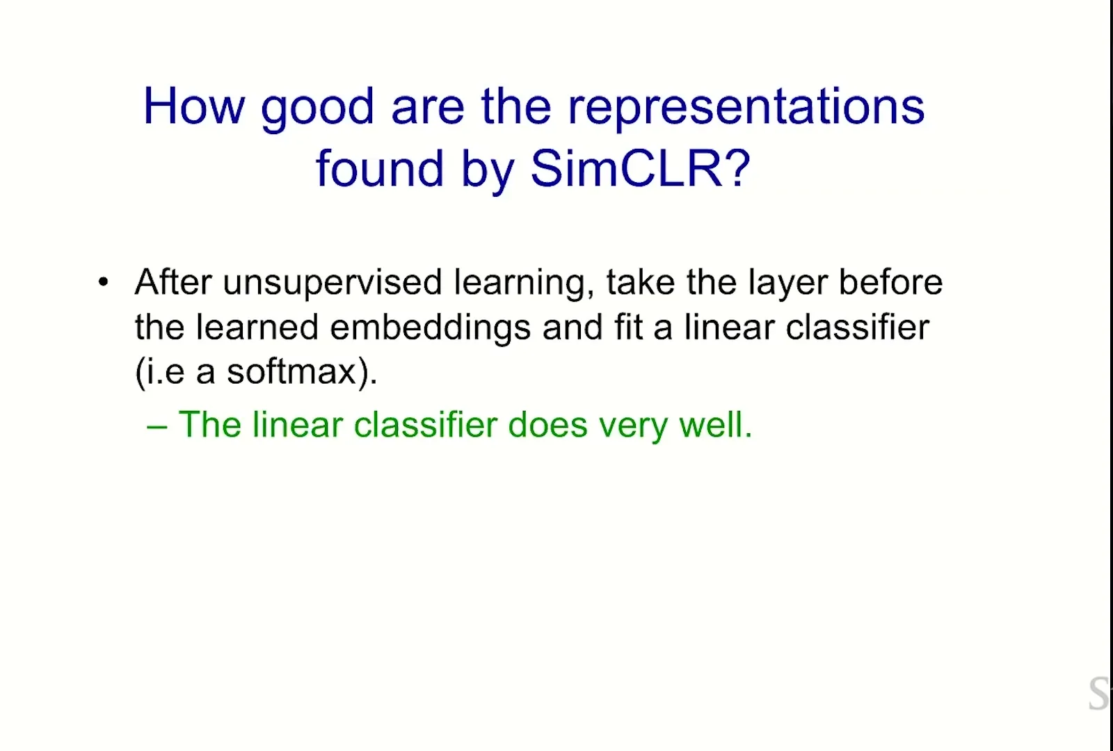
来源:Stanford Online 官方视频 00:25:08–00:28:11。
Linear probe 的正确读法
- probe 高:类别信息在 frozen representation 中近似线性可分;
- probe 低:可能是信息缺失,也可能是信息以非线性方式编码;
- probe 无法单独证明:对象边界、part-whole relation、pose equivariance 或 uncertainty calibration。
同图 crop 可能属于不同对象
如果一张街景同时有汽车、树和行人,把两块 crop 强行拉到同一 vector,可能只学到 scene identity,甚至抹掉 object distinction。GLOM 的目标是:在 scene level 可以大范围一致,在 object level 只让同一 object 的位置一致,在 part level 形成更小 islands。也就是说,agreement 的空间范围必须由 hierarchy 与 evidence 共同决定。
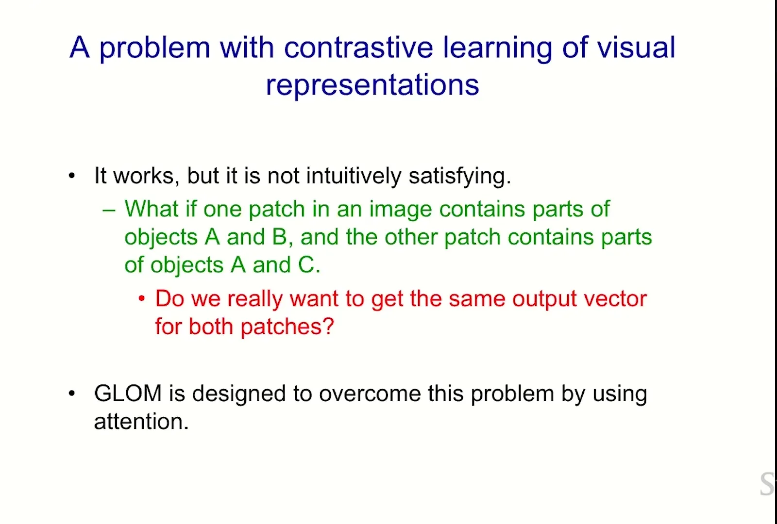
来源:Stanford Online 官方视频 00:28:12–00:28:49。
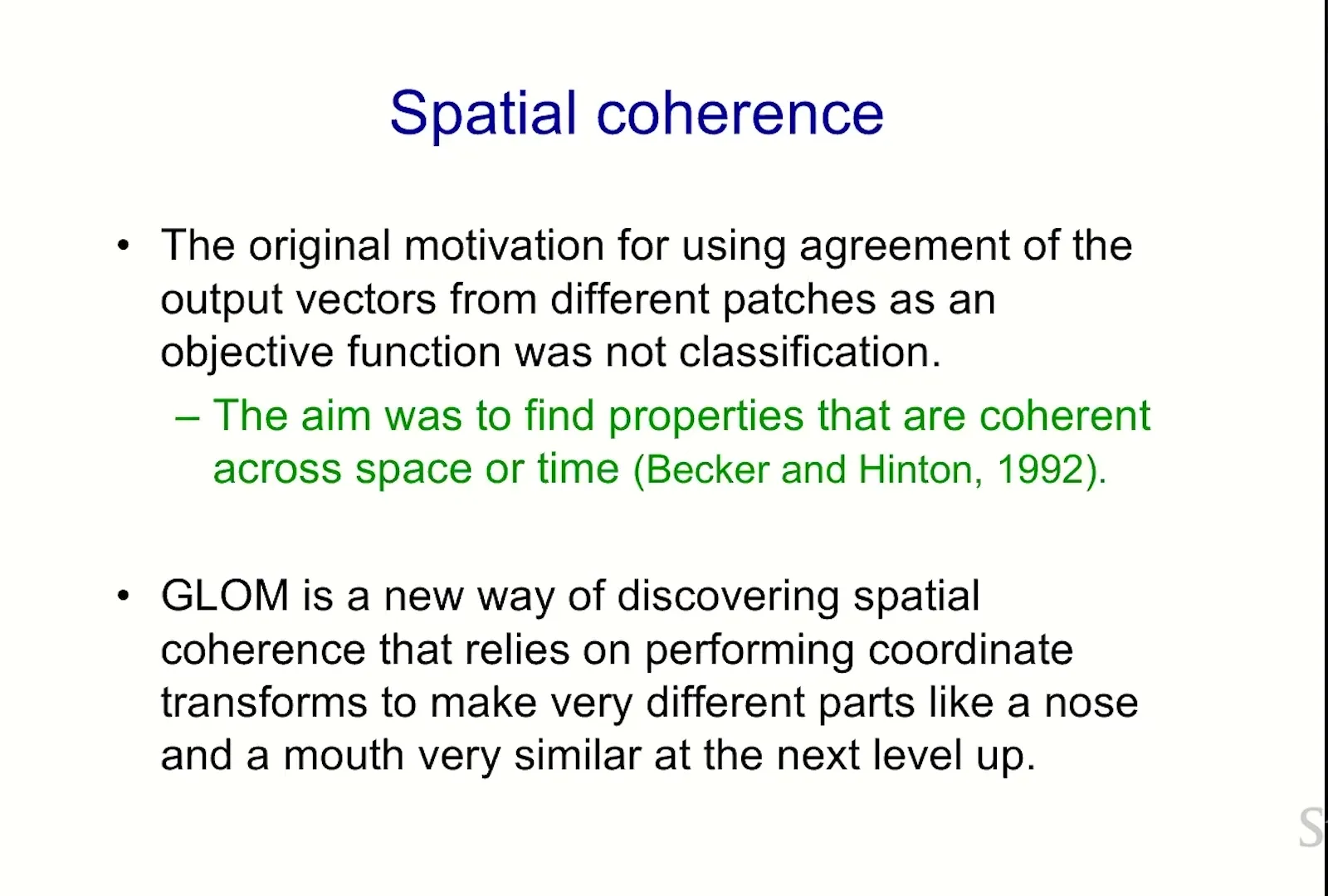
来源:Stanford Online 官方视频 00:28:50–00:30:17。
课堂提示
Hinton 把思路追溯到早期 spatial coherence work:相邻输出 vector 在真实表面或深度连续处应当一致。GLOM 的新问题是“不预先知道一致区域在哪里”,所以用 similarity attention 让 region 在 inference 中形成。
本章小结
Contrastive learning 教会我们:一致性 objective 可以学到强表示,但必须防 collapse,也必须说明“哪一级、哪些位置、在什么条件下应该一致”。GLOM 把这三个问题转交给 hierarchical state、coordinate prediction 与 local attention。
GLOM 的时空计算骨架
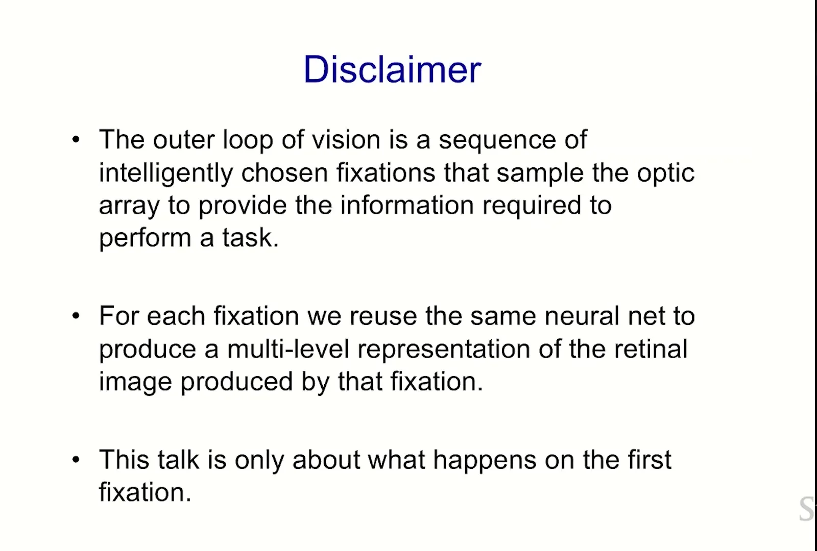
前几章回答“为什么需要这种表示”;现在进入可计算机制。GLOM 在每个空间位置、每个 hierarchy level 保存一个 embedding,并让这些状态跨若干 settling steps 更新。静态图像被视为重复帧的无聊视频,因此 temporal recurrence 仍然存在;真实主动视觉中的 fixation selection、foveation 与跨 fixation memory 则被暂时排除。
来源:Stanford Online 官方视频 00:30:18–00:34:29。
Scope omission:真实视觉不是一次全分辨率 forward pass
人眼中央高分辨率、外围低分辨率,并主动决定下一次看哪里;同一硬件会跨 fixation 重用。本讲把这些问题冻结,只讨论 first fixation 内的 recurrent settling。若把 GLOM 延伸到机器人或视频,policy、memory、motion correspondence 与 latency 都会重新出现。
状态张量与三个轴
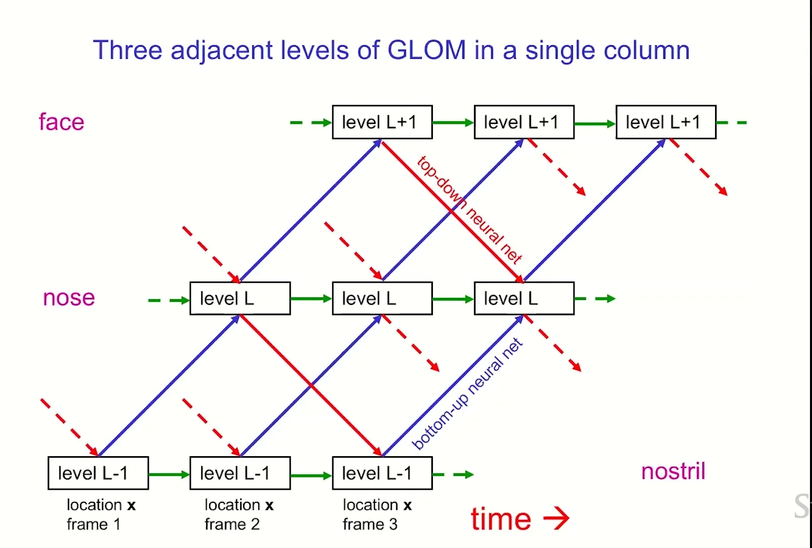
前面的 first-fixation 限制回答了“本讲暂时忽略什么”,现在需要回答“系统实际保存什么”。最关键的区分是 hierarchy level 与 settling time:前者描述 part-whole scale,后者描述同一输入解释被反复修正的过程;如果把二者都叫 layer,就会误读所有跨层和跨时箭头。可以把系统状态写成 \(\mathbf E^{(t)}\in\mathbb R^{|\mathcal X|\times(L+1)\times d}\):位置轴 \(x\)、hierarchy level 轴 \(\ell\)、settling time 轴 \(t\)。
来源:Stanford Online 官方视频 00:34:30–00:35:13。
读图:横向是 time,纵向是 hierarchy
每一列小方框属于同一 retinal location;从左到右是连续 settling steps,从下到上是 \(L-1,L,L+1\) 三个 part-whole levels。蓝箭头把低层上一时刻映射到当前层,红箭头把高层上一时刻映射下来,绿箭头保留同层历史,虚线斜向箭头表示与其他空间 columns 的 lateral interaction。图只画一个 location,因此 spatial neighborhood 必须结合下一张 slide 才完整。
课堂提示
讲者说 GLOM 本来是为 video 设计;静态图像只是每一帧都相同的“very boring video”。这句话解释了图中为什么同时出现 hierarchy 与 time,而不是把所有箭头误读成普通 network depth。
四个 contribution 的统一更新式
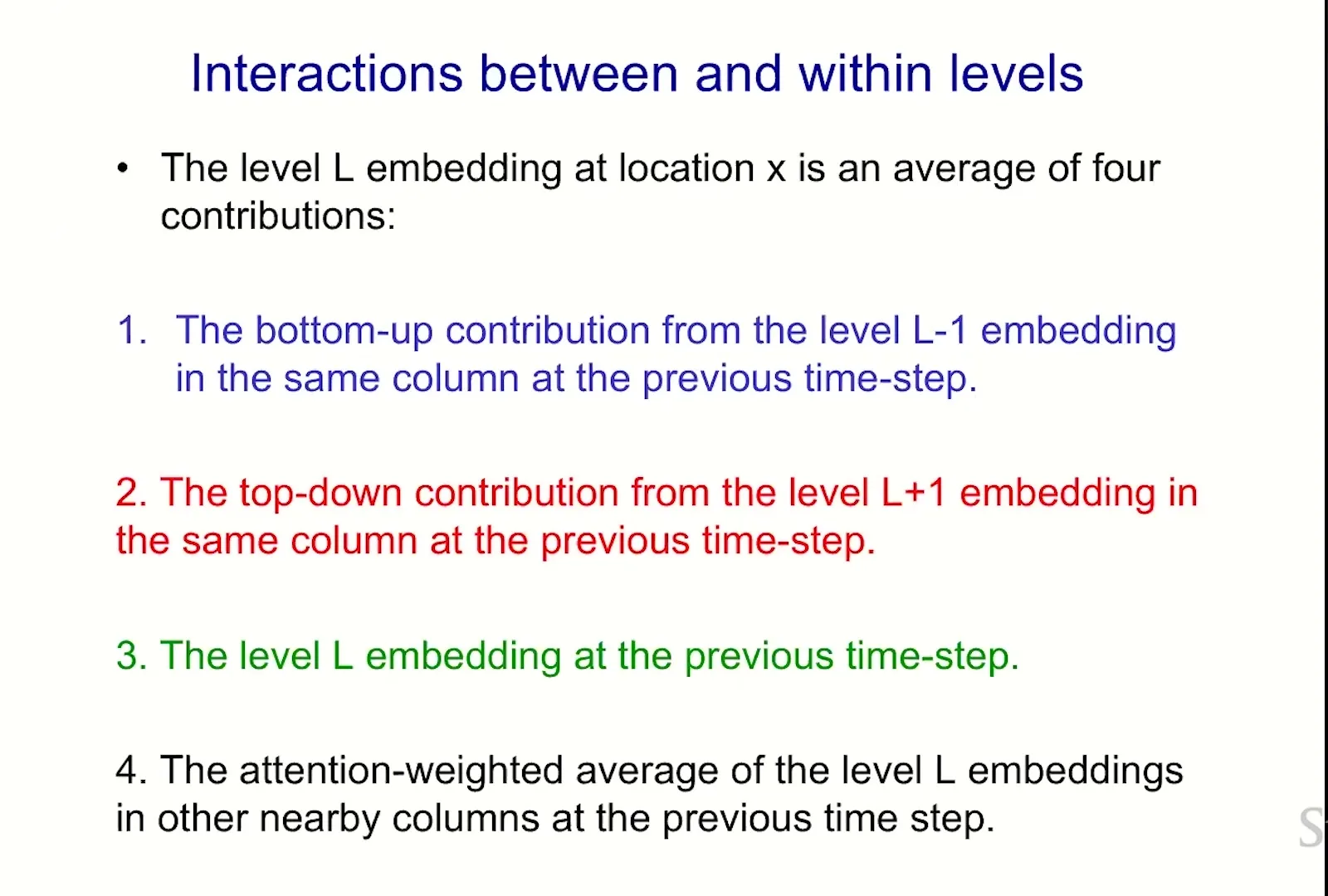
位置 \(x\)、层级 \(\ell\) 的下一状态由四类信息组成:低层向上预测、高层向下预测、同一状态的 temporal persistence、同层邻域的 attention consensus。一个教学化写法是:
其中,\(f_{\mathrm{bu}}^{\ell}\) 是 part-to-whole prediction,\(f_{\mathrm{td}}^{\ell}\) 是 whole-to-part prediction,\(x\) 可作为 neural-field location condition,\(\mathbf c_{x,\ell}^{(t)}\) 是 lateral consensus,四个 \(\lambda\) 表示随 level、time 或 reliability 调整的权重。课堂图说“average”,原论文进一步讨论 source reliability;这里的式子是机制归纳,不是唯一官方 implementation。
来源:Stanford Online 官方视频 00:35:14–00:35:47。
读图:四路输入分别承担不同责任
编号 1 的 bottom-up source 提供局部 evidence,编号 2 的 top-down source 提供 whole context,编号 3 的 previous-state source 提供 inertia,编号 4 的 neighborhood average 提供同层 agreement。它们不是四个可互换 residual branch:去掉 1 会脱离输入,去掉 2 会失去上下文修正,去掉 3 容易振荡,去掉 4 则无法让跨位置 hypothesis 形成 islands。
为什么 bottom-up / top-down 不是一根线
两条路径都需要 multi-layer neural network,因为它们不仅改维度,还要完成 identity 与 coordinate frame 的变换。相同 bottom-up function 应能处理 nostril-to-nose、steering-wheel-to-car 等不同类型;“universal”要求语义由 activity 决定,而非每种部件一套硬编码模块。
Similarity-gated lateral attention
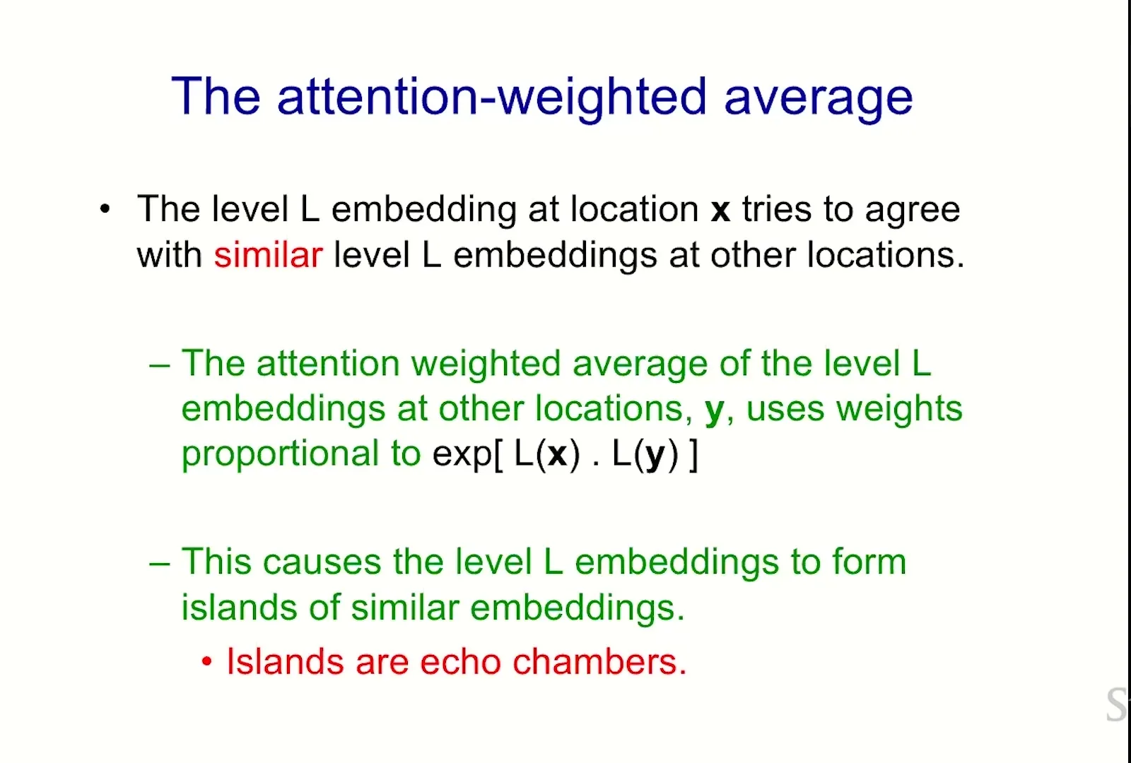
四路更新式仍留下一个关键问题:lateral branch 怎样区分“应当成为同一 island 的邻居”和“只是空间上靠近的另一个对象”?本节把这条选择规则展开,并说明 locality 与 temperature 为什么是 anti-collapse contract 的一部分。同层邻域 \(\mathcal N_\ell(x)\) 中,只有已经相似的 embedding 才强烈相互吸引;课堂给出的形式接近 dot-product softmax:
其中,\(\alpha_{xy}\) 是 \(y\) 对 \(x\) 的 lateral weight,\(\beta_\ell\) 控制 similarity sharpness,\(\mathcal N_\ell(x)\) 是 level-specific neighborhood,\(\mathbf c\) 是邻域共识。局部性很重要:若所有位置从一开始都全局互吸,global collapse 会成为更强 shortcut。
来源:Stanford Online 官方视频 00:35:48–00:37:13。
读图:红字“islands are echo chambers”既是机制也是风险
中心位置 \(x\) 先与邻域各位置比较 same-level embedding,相似者获得更大 softmax weight,再形成 weighted average。正反馈会让已有相似区域更一致,因此形成 island;但同一正反馈也可能把错误 hypothesis 放大。读图时应同时问三件事:neighbor range 多大、similarity 如何归一化、跨真实 boundary 的错误 attention 如何被 bottom-up evidence 拉回。
GLOM attention 与标准 Transformer 的差别
| 维度 | 标准 Transformer 常见设置 | 本讲 GLOM 草图 |
|---|---|---|
| Q/K/V | 可由不同投影产生 | 课堂把 embedding、key、query、value 极度简化为同一向量 |
| 范围 | 常见全局或预设 sparse pattern | level-specific local neighborhood;高层可更远、更稀疏 |
| 执行 | 固定层数的一次 forward | 同一输入上多次 recurrent settling |
| 目标 | token contextualization | 形成同层 islands,并与上下层 coordinate prediction 一致 |
def glom_step(state, level, neighbors, weights):
    next_state = {}
    for x in state.locations:
        current = state[x, level]
        lower = state[x, level - 1]
        upper = state[x, level + 1]

        bottom_up = bottom_up_net[level](lower)
        top_down = top_down_net[level](upper, location=x)

        scores = [dot(current, state[y, level]) for y in neighbors(x, level)]
        alpha = softmax(weights.beta[level] * scores)
        lateral = weighted_sum(alpha, [state[y, level] for y in neighbors(x, level)])

        mixed = (weights.bu * bottom_up + weights.td * top_down
                 + weights.self * current + weights.lat * lateral)
        next_state[x] = normalize(mixed)
    return next_state
本章小结
GLOM 的计算单元不是一个静态 block,而是 position、level、time 三维状态上的 recurrent consensus process。四路 update 同时携带局部 evidence、whole expectation、temporal inertia 与邻域 agreement;任何一路缺失,都可能让结构失去 pose、context、稳定性或边界。
Ambiguity:从 Pairwise Message 到 Hough-Style Voting
低层证据天然多义:一个 circle 可能是 left eye、right eye、front wheel 或 back wheel。若每个候选 part 都直接向所有其他候选 part 发送“你是否支持我”的 pose-transformed message,relation type 与 spatial pair 会快速膨胀。GLOM 提出另一种方向:让每个 part 都预测 parent identity-pose,再在 parent level 检查这些预测是否一致。
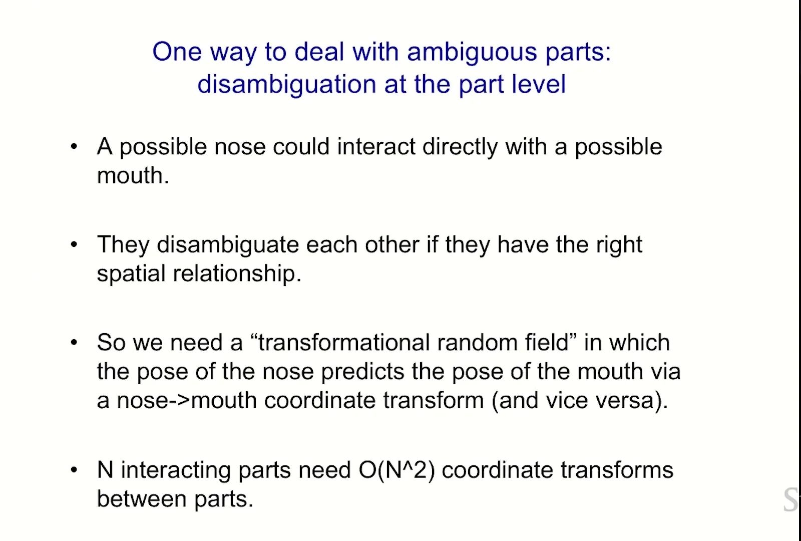
来源:Stanford Online 官方视频 00:39:04–00:43:35。
Transformational random field 的复杂度
假设 nose hypothesis 要询问附近是否存在兼容 mouth。message 不只说“有/没有 mouth”,还要把 nose pose 经 nose-to-mouth relation 变换成 expected mouth pose,回程再做 inverse transform。若 \(N\) 个候选位置、\(H\) 种 relation head 都直接交互,朴素 message 数量接近 \(O(HN^2)\),且每条 message 都含 coordinate transform。
这里的 \(O(N^2)\) 是设计压力,不是实测 profiler 数据
课堂用它说明 direct relation-specific messaging 为什么复杂。真实成本还取决于 local window、candidate pruning、head sharing、sparsity 与 representation dimension;不能据此直接给 GLOM 或 Hough route 做速度排名。
Hough transform:让 parts 在 parent space 会合
更简单的做法是:nose 与 mouth 不直接互认,而各自预测 face 的 identity 与 pose。如果两个不同位置、不同外观的 part 给出相同 parent embedding,那么 parent level 的 attention 会将其视为互相支持。这与经典 Hough voting 相似:局部 evidence 被映射到一个共同 hypothesis space,峰值代表一致解释。
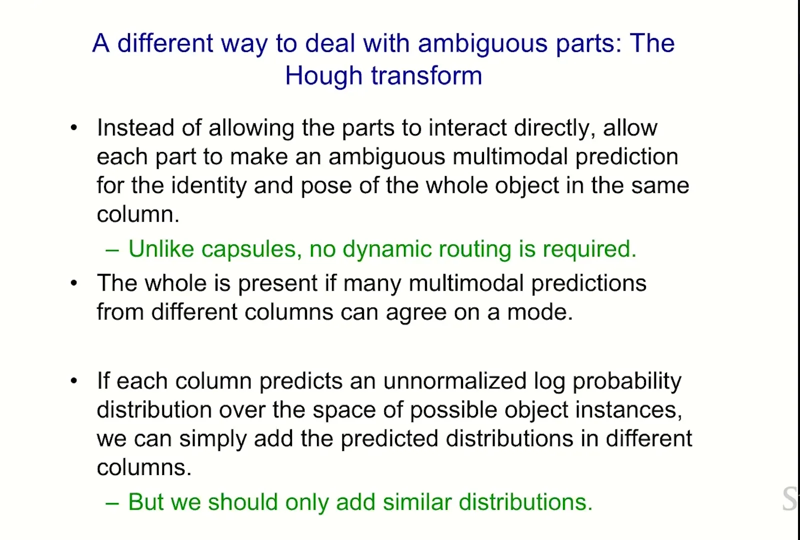
来源:Stanford Online 官方视频 00:43:36–00:44:31。
读图:比较 direct relation 与 common-parent vote
图左的 direct route 需要 nose 对不同潜在 mouth、eye 等发送 relation-specific message;图右把每个 part 映射到 whole hypothesis space。nose 与 mouth 虽位于不同 columns,只要预测出相同 face identity-pose vector,就会在 face level 相互支持。关键比较不是“有没有 attention”,而是 attention 发生在 pairwise part space 还是 common parent space。
可以把 part \(p\) 的 parent prediction 抽象为:
若 nose 与 mouth 属于同一 face,则理想情况是
其中,\(\mathbf e_p\) 包含 part identity 与 pose,\(f_{\mathrm{bu}}\) 学习 part-to-whole relation,\(\hat{\mathbf e}_w^{(p)}\) 是该 part 对 parent 的 vote。agreement 支持共同 parent,但 disagreement 也可能来自 occlusion、bad pose estimate 或多个重叠 objects。
为什么这条路线减少 routing burden
每个 column 的 embedding 始终描述该空间位置“在某层是什么”;column 内不需要把 activity 动态搬到另一颗专用 capsule。跨 column 的联系仍存在,但退化为 same-level similarity attention:比较的是 parent votes,而不是为每种 part-pair 建专用 routing table。
如何保留 multiple hypotheses
一个 circle 在 early inference 中不能立刻被压成唯一解释。Hinton 提出:embedding 中每个 neuron 对 joint identity-pose space \(z=(\text{identity},\text{pose})\) 提供一个宽的 log-probability basis function;多个 active neurons 的 contribution 相加后,可以形成尖锐或多峰分布。
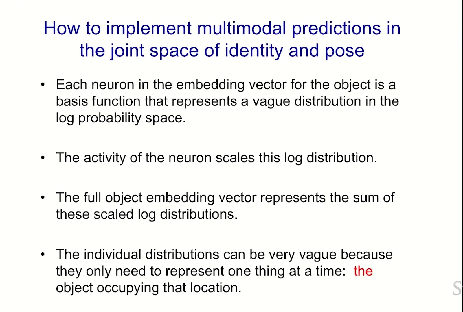
来源:Stanford Online 官方视频 00:44:32–00:44:45。
读图:vague basis 相加后才形成 sharp hypothesis
单个 neuron 对 joint identity-pose space 贡献一块宽的 log-probability surface,因此不能单独读成“这个 neuron 就是左眼”。多个 active basis 的加和相当于多个 constraints 的交集,可留下一个或多个峰。图没有展示 normalized probability、训练方式或 calibration;它只解释 distributed activity 如何在原则上保留 multiple hypotheses。
一个教学化表达是:
其中,\(z\) 是 identity-pose hypothesis,\(e_i\) 是 embedding 第 \(i\) 个 activity,\(\phi_i(z)\) 是该 neuron 在 hypothesis space 中的宽 basis function,\(Z(\mathbf e)\) 是 normalization constant。不同 evidence 的 log probability 相加,相当于 probability 相乘,可让重叠支持区域变尖。
讲者自己把这个论证称为 weak argument
这是一种 representational hypothesis:它说明 high-dimensional distributed activity 可能如何表达 multimodal uncertainty。课堂没有给出 calibrated likelihood、basis visualization、ablation 或 neural recording 来验证公式。讲义保留公式是为了让假说可检验,不是给它追加虚假的实证权威。
课堂提示
Hinton 说 perception 必须处理 uncertainty,因此 neuron 不能只代表一个确定对象;但他也承认“这是我能想到的唯一方式”并不是强证明。这个自我批评应与公式放在同一页,否则读者会把设计偏好误读成事实。
本章小结
GLOM 用 part-to-whole vote 把 relation-specific pairwise messaging 转换成 parent-level agreement;再用 distributed log-probability basis 为 early ambiguity 留空间。这两步都很有解释力,但分别需要 complexity experiment 与 uncertainty calibration 才能成为被验证的机制。
训练:Masked Reconstruction、Settling 与 Consensus Distillation
表示机制只有在 objective 能把正确 islands 学出来时才成立。课堂给出两类互补 signal:像 BERT 一样遮掉输入 patch、让系统经过若干 settling iterations 重建;再把 bottom-up/top-down predictions 拉向融合了邻域与时间信息的 consensus embedding,以鼓励局部一致区域形成。
Masked reconstruction 与 BPTT
给定图像 \(I\) 和 mask \(M\),输入中删除部分 patch。系统运行约 \(T\approx10\) 个 recurrent steps,再从最低层预测缺失内容。重建 loss 通过 time 与 hierarchy 反向传播,因此高层 hypothesis、低层 evidence 与 lateral agreement 都可能接收 gradient。
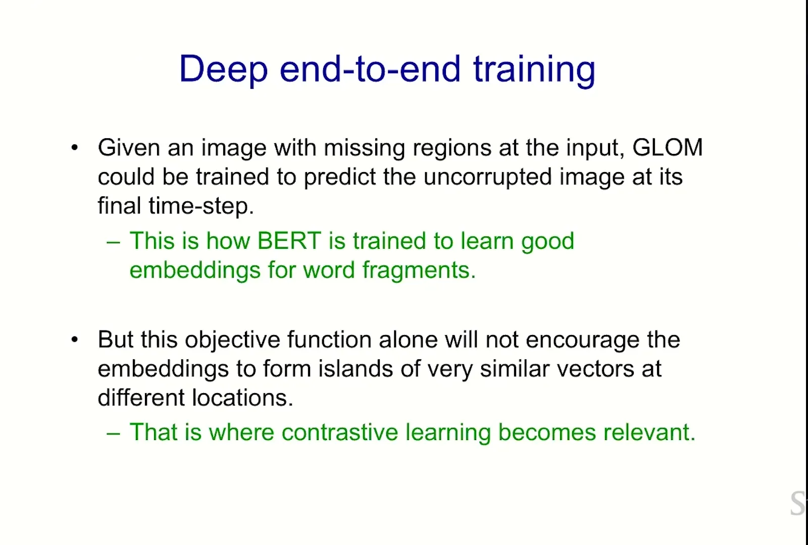
来源:Stanford Online 官方视频 00:44:46–00:45:43。
其中,\(M\) 是 masked locations,\(I_x\) 是真实 patch,\(D\) 是从最低层 embedding 重建输入的 decoder,\(T\) 是 settling steps,\(\ell\) 可是 pixel、feature 或 distribution loss。课堂没有固定唯一形式;重要的是 error 必须穿过 recurrent inference path。
“Train like BERT”并不意味着 optimization 一样简单
BERT 的 mask prediction 主要穿过固定深度 forward graph;GLOM 还要跨 settling time、上下 levels、attention neighborhoods 与 shared prediction nets 做 BPTT。梯度稳定、memory、truncation、fixed point 与 early-exit criteria 都是额外工程问题。
Consensus embedding 作为 teacher
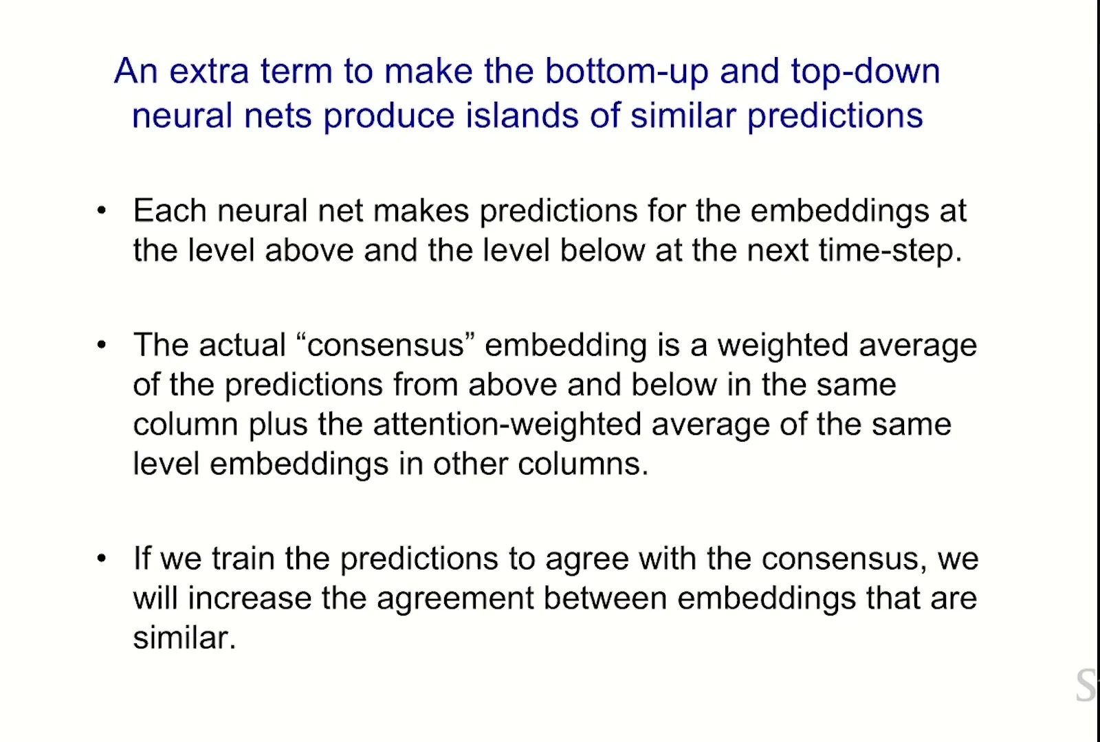
四路输入混合后的 target 被称为 consensus embedding。如果 bottom-up 与 top-down predictors 各自只看一种 source,它们可以被训练去逼近已融合相似邻域、前一时刻和另一层信息的 consensus。由于 lateral attention 已偏向 nearby similar states,逼近 consensus 会间接推动 island formation。
来源:Stanford Online 官方视频 00:45:44–00:47:11。
读图:teacher 不是标签,而是融合状态
bottom-up 与 top-down nets 各自给出 prediction;同层历史、邻域 attention 与其他方向的信息共同形成 consensus。训练把单源 prediction 拉向这个融合 target,因此不同 columns 可以交换知识。读图时必须保留两条限制:consensus 依赖当前模型自身,可能漂移;如果所有 peers 共享同一偏差,co-distillation 会强化而不是纠正错误。
设 \(\mathbf c_{x,\ell}^{(t)}\) 为 stop-gradient teacher,可写成:
其中,\(\operatorname{sg}\) 表示 stop-gradient,避免 teacher 与 student 同时沿同一路径任意漂移;两项分别训练 bottom-up 与 top-down predictor。论文也讨论不完全 weight sharing 的 biological variant;课堂图则更偏工程化共享模型。
Weight sharing 与 brain plausibility
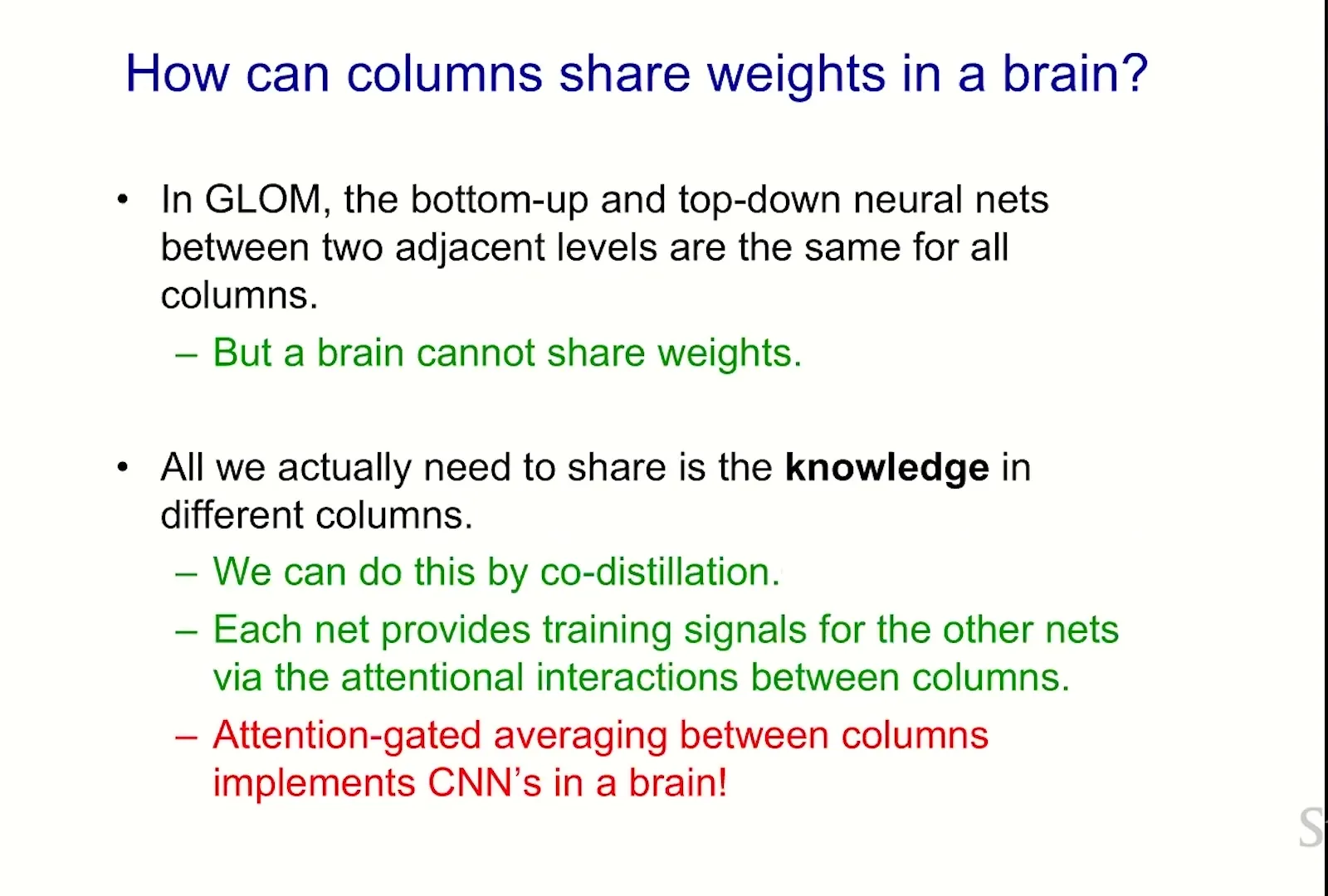
工程系统可以在所有位置复制同一 bottom-up/top-down weights;大脑未必精确共享权重。GLOM 论文提出 co-distillation:不同位置的 local models 即使参数略有差异,也可通过共同 consensus 交换知识。这个想法解释“功能近似共享”如何不依赖 exact parameter tying,但会引入 teacher quality 与 coordination 问题。
来源:Stanford Online 官方视频 00:47:22–00:48:51。
Distillation 术语消化
| 术语 | Teacher 从哪里来 | 在本讲中的作用 |
|---|---|---|
| knowledge distillation | 预训练大模型或 ensemble 输出 | 把 soft target 传给 student |
| online distillation | 训练中的 peers/ensemble 即时产生 target | 同步多个模型或分片的知识 |
| co-distillation | peers 互为 teacher,或 ensemble consensus 教所有 peers | 让不同 columns 的 predictors 向共同 island-compatible target 靠近 |
| consensus | temporal、bottom-up、top-down、lateral 信息的融合状态 | 不是 ground truth;可能放大共同错误 |
def train_step(image, mask, steps=10):
    visible = apply_mask(image, mask)
    state = initialize_columns(visible)

    consensus_targets = []
    for _ in range(steps):
        state, consensus = glom_step_all_levels(state)
        consensus_targets.append(stop_gradient(consensus))

    reconstruction = decode_lowest_level(state)
    reconstruction_loss = loss_on_masked_patches(reconstruction, image, mask)

    consensus_loss = 0.0
    for target in consensus_targets:
        consensus_loss += prediction_to_consensus_loss(state, target)

    total_loss = reconstruction_loss + CONSENSUS_WEIGHT * consensus_loss
    total_loss.backward()  # backpropagation through settling time
Consensus 也可能共同犯错
若初始 evidence 有偏、attention 过尖、邻域跨过真实边界,所有 predictors 可能朝错误 consensus 收敛。可靠系统需要 source weighting、uncertainty、boundary diagnostics、curriculum 或 alternative hypotheses,而不能把“大家同意”当成“大家正确”。
本章小结
训练提案把 masked reconstruction 提供的外部 error 与 consensus distillation 提供的内部结构信号结合起来。它说明 islands 可以如何被优化,但也暴露 GLOM 最难的工程部分:recurrent BPTT、teacher drift、collapse、边界泄漏与 settling stability。
Replication、Cluster Formation 与 Hierarchical Sparsity
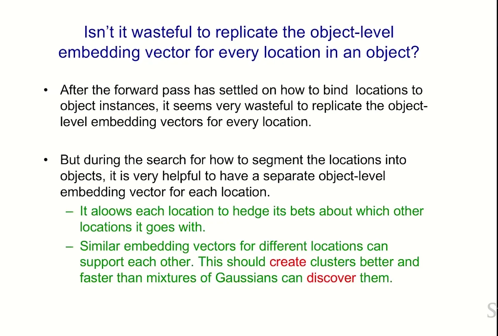
GLOM 会在一个 object 覆盖的许多位置复制同一高层 embedding,看起来非常浪费。Hinton 的反驳是:在 binding 尚未确定时,每个位置保留独立 hypothesis 才能逐步决定“哪些位置应该相同”;复制不是最终压缩最优,而是 inference flexibility 与 locality 的代价。
来源:Stanford Online 官方视频 00:48:52–00:49:47。
课堂提示
讲者用 biology 类比:细胞复制相同 DNA,器官不同部位也可有相近 protein-expression vector。这个类比的教学作用是说明 locality 可能值得冗余;它不是说 GLOM embedding 等同于基因或蛋白表达。
Forming clusters,不是对固定点做 clustering
普通 clustering 接收固定 data points,再发现分组;GLOM 中 data points 自己会随 bottom-up、top-down、lateral 与 temporal interaction 改变。系统不是对既有 embedding 聚类,而是在 recurrent dynamics 中共同形成 embedding 与 cluster boundary。
“Hedge your bets”的计算含义
在早期 step,位置 \(x\) 可以保留与邻居不同的 parent hypothesis;随着证据积累,兼容 positions 才被吸入同一 island。若一开始就把整块 object 压成单一 shared variable,错误 binding 很难局部修正。复制换来的是 delayed commitment。
动态形成不等于自动获得正确 discrete cluster
连续向量可能形成模糊过渡、多个局部 attractor 或 global consensus。若需要离散 object slot,还要定义 readout、threshold、connectedness、temporal tracking 与 birth/death rule。本讲并未完成这套 contract。
高层更远、更稀疏
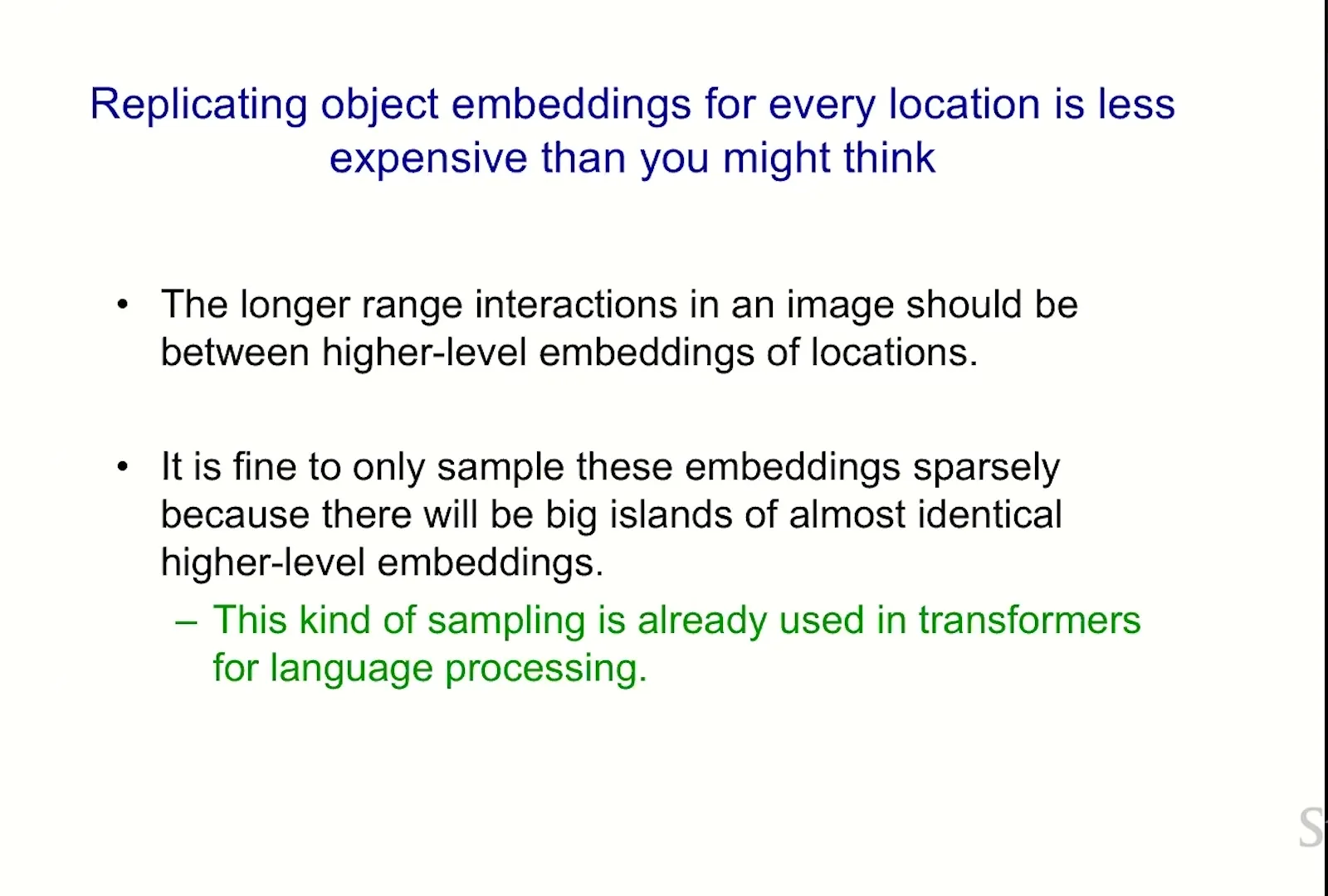
低层 part 小、边界细,需要短程 dense interaction;高层 object/scene island 大、内部冗余高,可以扩大 receptive radius,却只采样少数位置。目标是让 hierarchy level 上升时,communication range 增长而 edge count 不爆炸。
来源:Stanford Online 官方视频 00:49:48–00:50:07。
读图:range 增大不要求 edge count 同比例增长
高层 object island 覆盖许多 patches,内部向量预期高度冗余,因此一个位置不必连接 island 内所有位置;只要 sparse sample 命中代表点,就可能获得相同 whole hypothesis。图表达的是 range–density tradeoff:interaction radius 随 level 增长,连接密度下降。它没有给出 neighbor-search cost、miss rate 或实际吞吐量,所以只能作为 systems hypothesis。
| 层级 | 典型实体 | Interaction pattern | 主要风险 |
|---|---|---|---|
| 低层 | edge、texture、small part | 短程、较 dense,保护细边界 | 只看局部会错过 whole context |
| 中层 | major part、object component | 中程、按 similarity gated | 容易把相似但不同实例粘连 |
| 高层 | object、person、scene | 长程、较 sparse,利用大 island 冗余 | sparse sample 可能漏掉小对象或多实例冲突 |
“每层工作量相同”是目标,不是测量结果
要验证该主张,需要明确每层位置数、neighbor count、embedding width、迭代步数、routing/ANN search、memory traffic 与 communication pattern。单说“更 sparse”不足以证明 FLOPs、latency 或 energy 恒定。
本章小结
Embedding replication 为 gradual binding 与 local correction 保留自由度;hierarchical sparsity 试图把这种冗余转化为可扩展 interaction。两者共同体现 GLOM 的核心取舍:宁可在 state memory 上重复,也不提前把 uncertain structure 压成不可逆的单一 node。
Neural Field:同一个 Whole 如何生成不同 Parts
最后两分钟补上了一个容易被遗漏、却决定 top-down path 是否自洽的问题:若 face-level island 在所有位置都是同一 vector,而且所有 column 共享同一个 top-down network,为什么有的位置输出 nose、有的位置输出 mouth?答案是 top-down function 还接收 target location。
Location-conditioned top-down prediction
令 whole embedding 为 \(\mathbf e_w\),需要预测的位置为 \(x\),则 shared decoder 是函数
其中,\(\mathbf e_w\) 同时编码 whole identity 与 pose,\(x\) 指定要查询的图像位置,输出是在该位置应出现的 lower-level identity-pose embedding。相同 face vector 配合不同 \(x\),可以生成 nose、mouth 或其他 part prediction;这就是 coordinate-conditioned neural field 的基本形式。
课堂提示
Hinton 先提出一个表面矛盾:red arrows 与 green arrows 完全不同,上层 face vectors 却相同;如果 top-down weights 也共享,怎么产生不同结果?他的解答是把 query location 一并输入。这个补充把“共享权重”从口号变成了函数签名。
Neural field 在这里解决什么
- 输入:whole identity/pose embedding 加 target coordinate;
- 输出:该 coordinate 上的 lower-level prediction;
- 价值:共享同一 decoder,却能在不同位置产生不同部件;
- 不等价:课堂并未要求使用 NeRF 的 volume rendering、ray sampling 或 photometric loss。
与现代 coordinate-conditioned model 的连接
NeRF、implicit neural representation、一些 world model decoder 都使用“global/local latent + coordinate/query”产生位置特定输出。GLOM 的独特点在于 decoder 不是只从一个 global latent 渲染像素,而嵌在多层 recurrent islands 中:top-down prediction 必须与 bottom-up evidence、lateral agreement 和 temporal state 共同收敛。
Connection 不是 lineage claim
把 GLOM 与现代 object-centric decoder、slot model、world model 相连,是工程解释;不能说后者“实现了 GLOM”,除非它们真的满足 island representation、multi-level recurrence、four-source consensus 与 coordinate-aware part-whole prediction 等更强条件。
本章小结
Location condition 解决了 shared top-down network 的表达矛盾:同一个 whole representation 可以针对不同坐标发出不同 part prediction。它也是整套设计中最接近成熟现代技术的组件,但 GLOM 的难点仍在于如何把该 decoder 与动态 islands 稳定联合训练。
系统级复盘:GLOM 到底组合了什么
走到这里,可以把 GLOM 压成一个 recurrent structured inference loop:低层 evidence 向上提出 parent hypothesis,高层 context 向下预测 part,same-level attention 让相似 hypothesis 形成 islands,previous state 提供 inertia,masked reconstruction 与 consensus distillation 训练这些函数,location-conditioned decoder 处理 shared whole 到不同 parts 的生成。
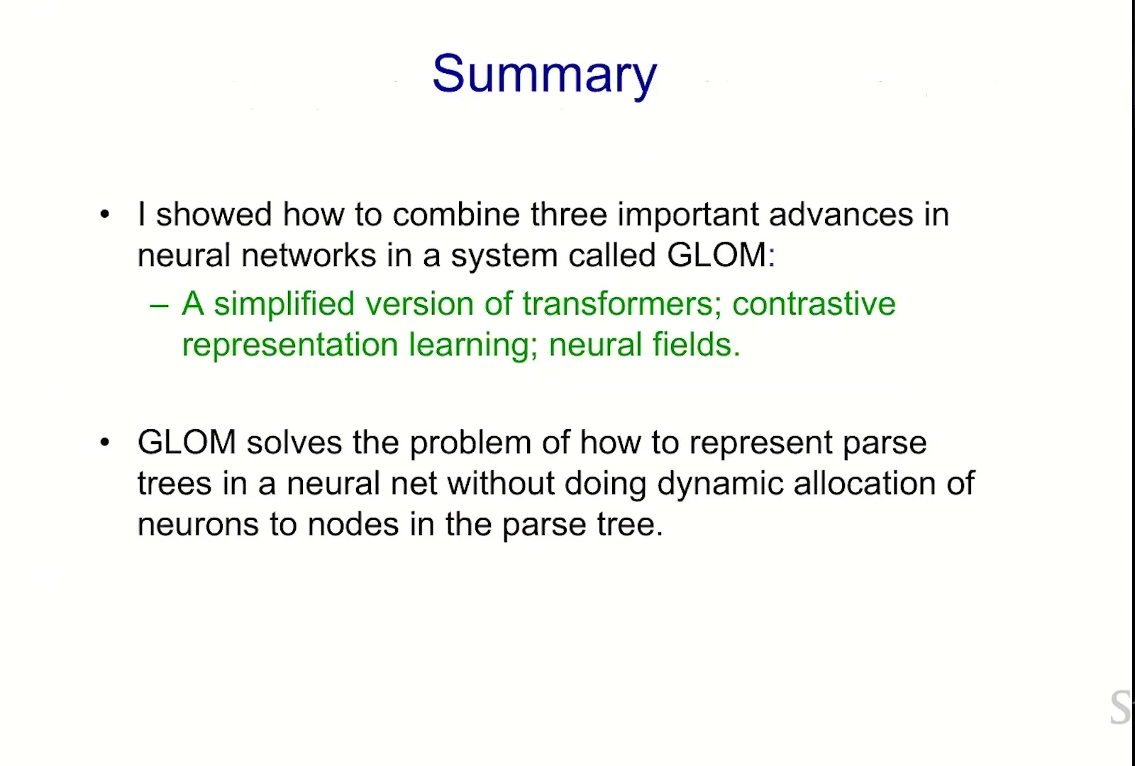
来源:Stanford Online 官方视频 00:50:08–00:52:20。
机制清单与失败模式
| 机制 | 试图解决的问题 | 尚缺的验证 |
|---|---|---|
| Dynamic embeddings | 固定硬件表示输入特定 parse | 与 ground-truth hierarchy 的 alignment |
| Islands of agreement | 用相同 activity 表示同一 node | 防 collapse、跨实例分离、边界稳定性 |
| Bottom-up/top-down maps | part-whole identity/pose consistency | coordinate equivariance 与 occlusion robustness |
| Local similarity attention | 发现 spatial coherence region | attractor、error propagation 与 convergence |
| Hough-style parent voting | 避免 pairwise relation routing explosion | 对复杂 scene、多实例与 deformable object 的效果 |
| Consensus distillation | 让 local predictors 共享结构信息 | teacher drift、错误共识与 optimization stability |
| Sparse upper levels | 扩大 range 而控制 cost | 实际 FLOPs、memory、latency 与 communication |
| Neural field decoder | 相同 whole 在不同位置预测不同 parts | 与 islands 联合训练后的生成质量 |
读论文时应追问的实验
若今天把 GLOM 从 design document 推向系统论文,至少需要以下实验闭环:
- Representation readout:定义如何从连续 embeddings 提取 nodes、edges、identity 与 pose;
- Causal use:干预某个 island 后,验证对应 part/whole prediction 是否按结构变化;
- Convergence:测 settling steps、fixed-point stability、oscillation 与 early stopping;
- Anti-collapse:比较 local attention、negative pairs、variance regularization 与 consensus weighting;
- Generalization:测试新 viewpoint、新 part composition、occlusion、multiple instances 与 video tracking;
- Systems accounting:报告 state memory、attention edges、BPTT activation、wall-clock latency 与 energy;
- Ablation:分别移除 top-down、bottom-up、persistence、lateral attention、location condition 与 distillation。
一个可证伪的 GLOM 主张
若 islands 真正承担 parse-tree node,移除或扰动某个 parent-level island,应系统性改变其 constituent parts 的 top-down prediction,而不只是降低全局分类分数。这个 intervention 比“可视化看起来像 object”更接近机制证据。
本章小结
GLOM 的强项是把 representation、inference、learning 与 coordinate generation 放进同一设计语言;弱项是几乎每条关键链路都缺少端到端实验。正因为证据不完整,它特别适合作为 architecture thinking exercise:强迫读者把“对象结构”从直觉词汇改写成 state、message、loss 与 verification contract。
总结与延伸
本讲从一个简单但尖锐的问题出发:固定连接的神经网络如何表示每张输入都不同的 part-whole hierarchy?GLOM 的答案是,不动态分配 node hardware,而让 position-by-level grid 中的 activity 经过 recurrent interaction 形成 islands;同一 island 的近似一致向量代表一个 parse node,上下层 learned functions 表达 part-whole prediction,lateral attention 表达同层 agreement,location-conditioned neural field 让相同 whole 在不同位置生成不同 parts。
把整讲压成六个因果步骤
- Dynamic state replaces dynamic memory allocation:输入特定结构写进 activity,而不是改 weights;
- Coordinate-aware prediction proposes hierarchy:parts 向上投票 whole,whole 向下预测 parts;
- Local similarity attention forms islands:已相似的 same-level hypotheses 互相加强;
- Recurrent settling delays commitment:多步 inference 允许 ambiguity、修正与 top-down feedback;
- Reconstruction and consensus train the loop:外部 prediction error 与内部 co-distillation 共同塑造表示;
- Location-conditioned decoding preserves weight sharing:同一 whole vector 针对不同 coordinate 产生不同输出。
最终教学结论
GLOM 最值得保留的不是某个尚未验证的 update rule,而是一套 representation discipline:如果你声称模型理解对象结构,就必须说明 node 存在哪里、part-whole relation 如何编码、ambiguity 如何保留、binding 如何形成、结构如何被 loss 训练、以及哪些 intervention 能证明该结构真的被下游计算使用。
六个常见误区
不要把设计提案写成成功史
- 不要说 GLOM 已经解决 object-centric vision;本讲没有完整 benchmark;
- 不要把二维箭头当成真实 embedding dimension 或显式 pose matrix;
- 不要把 island 直接等同于 ground-truth segmentation mask;
- 不要把 consensus 等同于 truth,agreement 也可能是 shared error;
- 不要把 Hough analogy 当成已证明的 complexity advantage;
- 不要把 location-conditioned decoder 等同于完整 NeRF/modern world model。
面向现代系统的谨慎连接
今天的 object-centric representation、slot-based model、iterative refinement、equivariant network、implicit neural representation、video world model 与 sparse hierarchical attention 都触碰了 GLOM 的局部问题。真正有价值的比较不是看名字,而是逐项检查:是否有动态 entity state,是否显式处理 pose,是否保留 multiple hypotheses,是否允许 top-down correction,是否存在可读出的 part-whole relation,以及结构是否通过 causal intervention 被验证。
课堂提示
结束前 Hinton 说这是一场复杂的 talk,最好的用途可能是鼓励大家去读长论文。这个结尾与开场的 “vaporware” 呼应:他不是宣布问题已解决,而是在邀请读者把一个 representation idea 变成更严格的模型与实验。
拓展阅读
| Hinton, GLOM:完整设计文档。 | Sabour et al., Capsules:routing 背景。 |
|---|---|
| Chen et al., SimCLR:contrastive scaffold。 | Vaswani et al., Transformer:attention 基线。 |
| Devlin et al., BERT:masked reconstruction。 | Anil et al., Online Distillation:co-distillation。 |
| Mildenhall et al., NeRF:coordinate-conditioned field。 |