CS336 2026 Lecture 2：Resource Accounting、Tensor、FLOPs 与 Memory

LaTeX 源码 · 备用 PDF · 观看视频

字段	内容
作者/整理	基于 Stanford CS336 Spring 2026 官方可执行讲义整理
来源	Stanford CS336
日期	2026 年春季

本讲主线：resource accounting 是训练前的账本

Lecture 2 的目标是把“训练一个模型”拆成可估算的资源账本。语言模型训练不是只写 forward，而是在 compute、memory、bandwidth、dtype、optimizer state、activation 和 wall-clock time 之间做取舍。第一讲说核心目标是 efficiency；第二讲给出 efficiency 的基本单位。

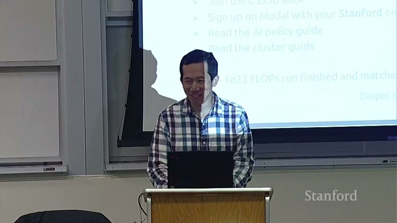
课程开场提到 Marin 的 \(10^{23}\) FLOPs run 已完成并匹配 forecasts。这不是新闻八卦，而是一个工程信号：scaling forecast 只有在 compute 和 memory 账本可靠时才可信。

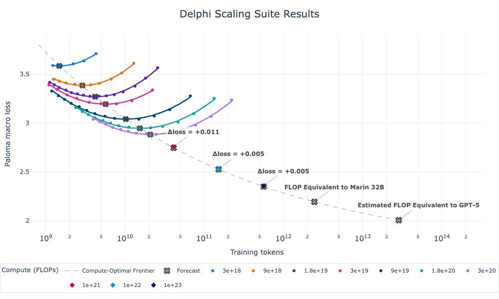
读图：Marin 结果图为什么放在 Lecture 2 开头

这张图展示的是“训练前预测”和“训练后观测”的闭环。要让这件事有意义，必须知道训练到底用了多少 FLOPs、硬件给了多少有效 FLOP/s、模型和 optimizer state 是否能放进显存、训练中是否有通信和 checkpoint 开销。Lecture 2 就是为这种预测能力补上底层账本。

两个 motivating questions

本讲先用两个问题训练数量级直觉。

\[ C_{\text{train}}\approx 6ND. \]

这里 \(N\) 是参数量，\(D\) 是训练 token 数，系数 6 来自 forward 约 \(2ND\) FLOPs、backward 约 \(4ND\) FLOPs 的粗略估计。70B 参数、15T token 的训练计算量约为：

\[ 6\times 70\times 10^9\times 15\times 10^{12} =6.3\times 10^{24}\ \text{FLOPs}. \]

若用 1024 张 H100，dense bf16 峰值约 \(989.5\) TFLOP/s，假设 MFU 为 0.5，则训练约需 140 多天量级。这不是精确排期，而是训练前判断可行性的 napkin math。

first-use glossary：FLOPs、FLOP/s、MFU

FLOPs 是 floating-point operations，表示总计算量；FLOP/s 是每秒浮点运算数，表示速度。MFU 是 model FLOPs utilization，即实际模型 FLOP/s 除以硬件承诺峰值 FLOP/s。训练时间约等于总 FLOPs 除以有效 FLOP/s。

第二个问题是 8 张 H100 用 AdamW 能训练多大模型。H100 每张约 80GB，8 张总 640GB。若每个参数需要 bf16 参数 2 bytes、bf16 gradient 2 bytes、AdamW 一阶动量 4 bytes、二阶动量 4 bytes，那么仅参数相关状态就要：

\[ 2 + 2 + 4 + 4 = 12\ \text{bytes/parameter}. \]

640GB / 12 约为 53B 参数。这还没算 activation memory、temporary buffers、CUDA workspace 和 fragmentation，所以是乐观上界。

参数上界不是可训练模型大小

如果不考虑 activations，你会系统性高估能训练的模型规模。大 batch、长 sequence、深层网络都会让 activation memory 迅速变成主要瓶颈。

first-use glossary：optimizer state

Optimizer state 是优化器为每个参数额外维护的状态。Adam/AdamW 通常维护 \(m\) 和 \(v\)：\(m\) 是梯度的一阶动量，\(v\) 是梯度平方的二阶动量。它们从零初始化，每步由新 gradient 更新。因为 \(m\) 和 \(v\) 通常用 fp32 存储，Adam 的 optimizer state 显存常常是参数本身的 4 倍（两个 fp32 state vs 一个 bf16 参数）。

first-use glossary：sharding 与 ZeRO

Sharding 是分片：原本每张 GPU 都保存完整对象，分片后每张 GPU 只保存一部分。ZeRO 是 Zero Redundancy Optimizer，在 data parallel 框架内把 optimizer state、gradients、parameters 分阶段切分。ZeRO-1 切 optimizer state，ZeRO-2 再切 gradients，ZeRO-3 连 parameters 也切。越省显存，通信越多。

本章小结

Resource accounting 的第一步是把模糊问题改写为数量级问题：需要多少 FLOPs？硬件有效速度是多少？哪些状态占显存？activation 是否被漏算？这些问题答不出来，就不应该启动大训练。

Tensor 与 Memory：所有训练状态都在张量里

Tensor 是训练系统的基本载体。Data、parameters、gradients、optimizer state、activations 都是 tensor，只是生命周期不同。

状态	什么时候存在	资源含义
Data	每步 batch 输入	影响 batch size、sequence length、host-to-device 传输。
Parameters	全程存在	模型权重，forward/backward/optimizer 都要访问。
Gradients	backward 后到 step 前	默认累积，需要及时清理或分片。
Optimizer state	多个 step 间长期存在	AdamW 的 \(m,v\) 等统计量，常是显存大头。
Activations	forward 后到 backward 用完	随 batch、sequence、layers 增长，可用 checkpointing 处理。

Transformer 中常见 rank-4 tensor：

\[ x\in\mathbb{R}^{B\times S\times H\times D}, \]

其中 \(B\) 是 batch size，\(S\) 是 sequence length，\(H\) 是 number of heads，\(D\) 是 head dimension。

shape ledger

Shape 不是注释，而是资源账本。\(B\) 增大会提升吞吐但增加 activation memory；\(S\) 增大会提高 attention 和 KV cache 成本；\(H,D\) 改变 attention/MLP 矩阵形状；\(L\) 影响参数、activation 和 checkpointing tradeoff。

数值格式：fp32、fp16、bf16、fp8、fp4

Tensor memory 由元素个数和 dtype 决定：

\[ \text{memory}(x)=\text{numel}(x)\times \text{element\_size}(x). \]

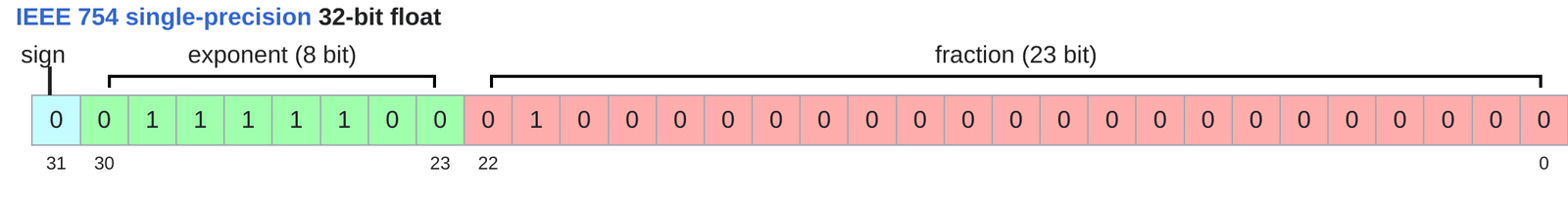
读图：fp32 为什么稳

fp32 有较大的 exponent 和 mantissa，动态范围和精度都充足，所以传统科学计算和 optimizer state 常用它。缺点是每个值 4 bytes，显存和带宽成本高。

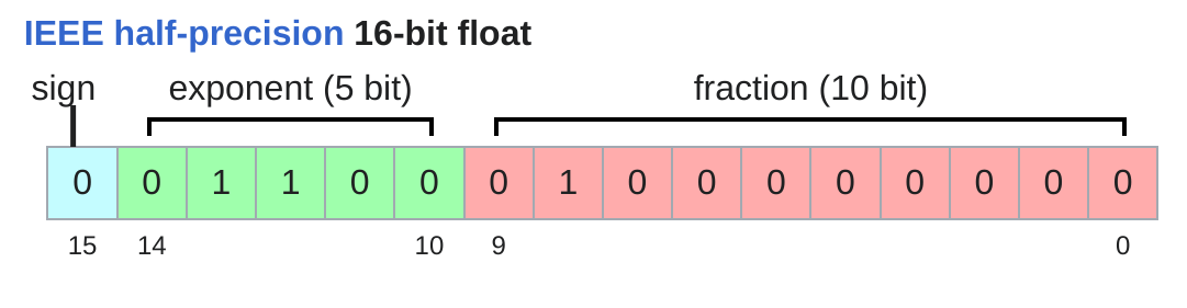
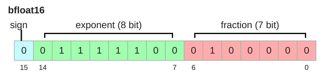
读图：fp16 与 bf16 的差别

fp16 给 mantissa 更多位，数值更细，但动态范围窄；bf16 给 exponent 更多位，动态范围接近 fp32。深度学习训练更怕数值下溢/溢出，因此 bf16 常比 fp16 更稳。

mixed precision 不是简单全改低精度

训练常用 bf16 存 parameters、activations、gradients，但 optimizer state 保留 fp32。这样省显存和带宽，同时让长期统计量保持稳定。

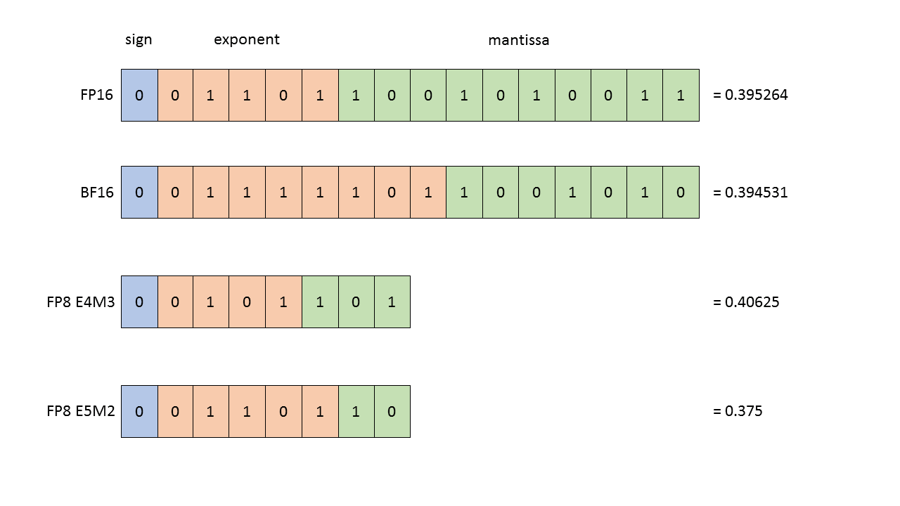
读图：为什么 FP8 有两个格式

E4M3 用 4 位 exponent 和 3 位 mantissa，精度相对好但范围小；E5M2 范围更大但精度更粗。FP8 能否有效使用，取决于硬件、scale 管理和库支持，不只是 dtype 名字。

FP4/NVFP4 进一步把每个值压到 4 bits，通常需要 block-wise scale 扩展动态范围。它更像高度优化库中的系统能力，而不是普通 PyTorch 默认路线。

CPU 与 GPU memory

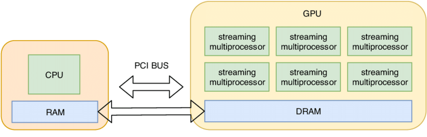
读图：CPU-GPU 图的系统含义

.to(device) 不是语法细节，而是数据移动。大模型训练中，CPU/GPU、GPU/GPU、HBM/SM 之间的每次移动都可能成为瓶颈。Lecture 2 从这里开始把 tensor 运算变成硬件数据流问题。

本章小结

Memory accounting 从 tensor、shape、dtype、device、生命周期开始。低精度能节省显存，但必须理解动态范围；GPU 能提供并行性，但前提是数据在正确位置，并且移动成本可控。

Einops 与 Shape：让维度变成可读账本

PyTorch 的 transpose(-2, -1)、sum(dim=-1) 很强，但隐藏了维度语义。Einops 用命名维度写 tensor operation，让表达式更接近数学。

传统 PyTorch 写法容易隐藏维度含义

x = torch.ones(2, 2, 3)      # batch seq hidden
y = torch.ones(2, 2, 3)      # batch seq hidden
z = x @ y.transpose(-2, -1)  # batch seq seq

Einops/einsum 用名字表达维度收缩

z = einsum(
    x, y,
    "batch seq1 hidden, batch seq2 hidden -> batch seq1 seq2"
)

术语消化：einsum、reduce、rearrange

• einsum：按名字指定哪些维度相乘、哪些维度求和、哪些维度保留。
• reduce：沿某些维度做 sum/mean/max/min。
• rearrange：拆分、合并、重排维度，例如把 total_hidden 拆成 heads hidden。

Shape 错误是隐性 bug

维度顺序错了，代码可能仍能运行，只是语义错。命名维度能减少这类错误，也为 tensor parallelism、sequence parallelism 和 attention head 切分打基础。

本章小结

Einops 代表一种资源核算习惯：每个维度都要有名字。后续计算 FLOPs、activation memory 和 parallelism 时，维度语义比张量本身更重要。

Compute Accounting：FLOPs、FLOP/s 与 MFU

FLOPs 与 FLOP/s

术语	含义	例子
FLOPs	floating-point operations，计算总量	GPT-3 训练约 \(3.14× 10^23\) FLOPs。
FLOP/s	每秒浮点运算数，硬件或程序速度	H100 dense bf16 峰值约 \(989.5\) TFLOP/s。
MFU	actual FLOP/s / promised FLOP/s	模型实际吃满硬件的程度，0.5 已经很好。

\[ \mathrm{MFU}=\frac{\text{actual FLOP/s}}{\text{promised FLOP/s}}. \]

FLOPs 和 FLOP/s 混淆会毁掉估算

FLOPs 是路程，FLOP/s 是速度。训练时间约等于总 FLOPs 除以有效 FLOP/s。有效速度又取决于 dtype、kernel、通信、shape 和 MFU。

矩阵乘法 FLOPs

若 \(X\in\mathbb{R}^{B\times D}\)，\(W\in\mathbb{R}^{D\times K}\)，则

\[ Y=XW,\qquad \text{FLOPs}\approx 2BDK. \]

每个输出元素需要 \(D\) 次乘法和约 \(D\) 次加法。实际程序还要 benchmark 得到运行时间，再算实际 FLOP/s。

MFU 的正确使用

MFU 不是道德评分，而是诊断工具。MFU 低可能是 memory-bound、通信同步、kernel 太小、shape 不友好、数据加载慢，也可能是测量口径不一致。下一节 arithmetic intensity 会解释其中最常见的一类原因。

本章小结

Compute accounting 的步骤是：从 shape 算 FLOPs，用 benchmark 得实际时间，再与硬件峰值比较。不要只数 FLOPs，还要问这些 FLOPs 是否能高效喂给硬件。

Arithmetic Intensity 与 Roofline

compute-memory 最小模型

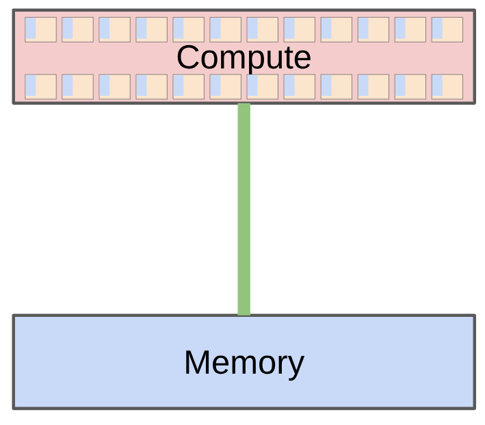
读图：compute-memory 图怎么连接到 roofline

如果每搬 1 byte 数据只做很少计算，硬件主要等 memory；如果每 byte 能复用很多次，硬件才可能接近 compute 峰值。Arithmetic intensity 就是把计算和数据移动放到同一张账本上。

\[ \text{arithmetic intensity} = \frac{\text{FLOPs}}{\text{bytes transferred}}, \qquad \text{accelerator intensity} = \frac{\text{peak FLOP/s}}{\text{memory bandwidth}}. \]

对 H100 dense bf16，峰值约 \(989.5\times 10^{12}\) FLOP/s，HBM bandwidth 约 \(3.35\times 10^{12}\) bytes/s，所以平衡点约 \(295\) FLOPs/byte。

判断瓶颈的规则

Workload intensity 小于 accelerator intensity，则 memory-bound；大于 accelerator intensity，则 compute-bound。

操作	intensity 直觉	LLM 对应场景
ReLU / elementwise	每个元素少量计算但完整读写 tensor	activation、mask、small kernels，常 memory-bound。
GeLU	比 ReLU 多算一些，但读写相同	单独 kernel 仍常 memory-bound。
Dot product	有 reduction，但复用有限	attention/normalization 的局部构件。
Matrix-vector	读大矩阵服务少量 token	autoregressive decode 常见。
Matrix-matrix	数据复用高，intensity 随规模增长	training/prefill 中的大 matmul。

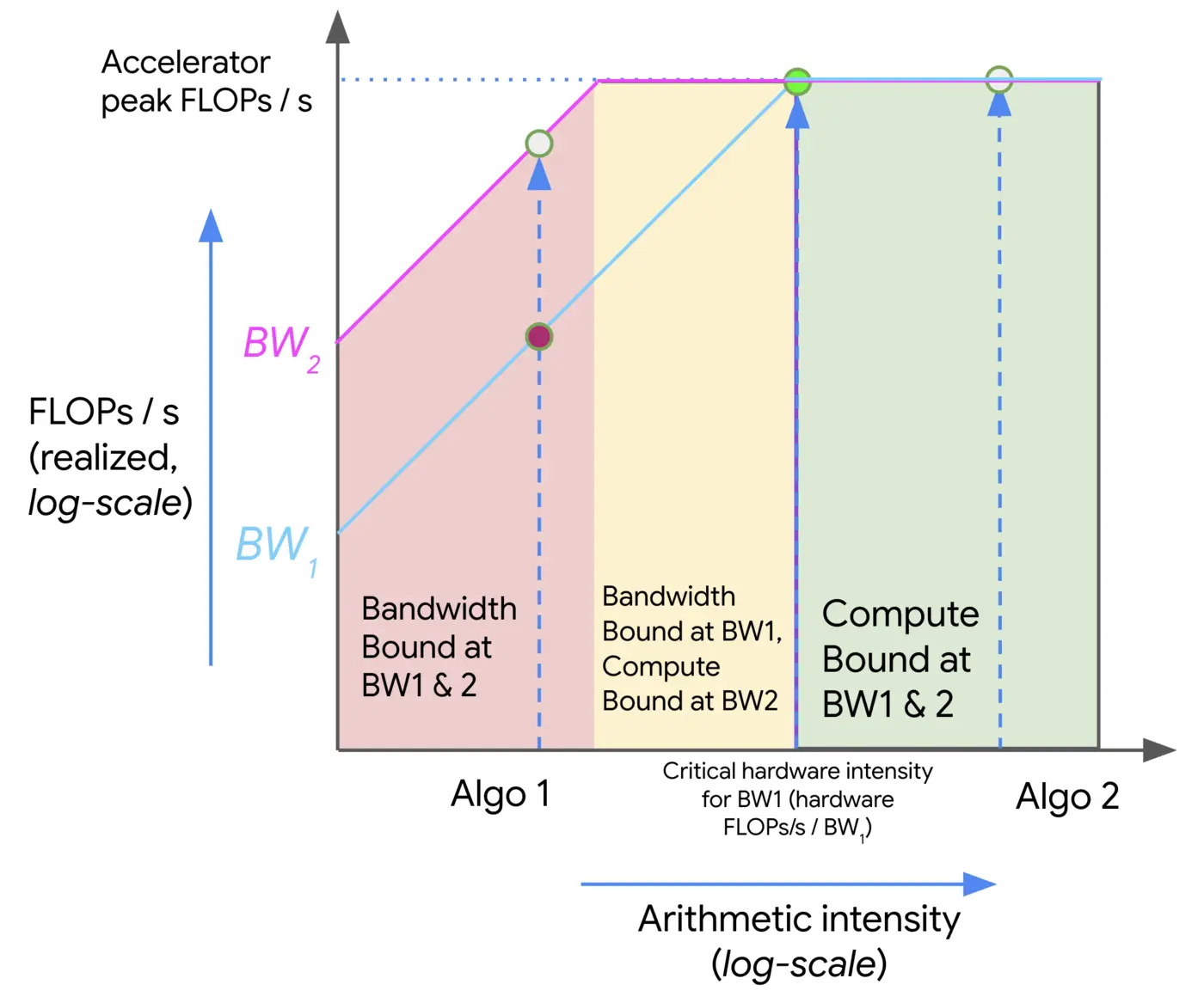
读图：roofline plot 怎么看

横轴是 arithmetic intensity，纵轴是可达 performance。左侧斜线由 memory bandwidth 限制，右侧平台由 peak FLOP/s 限制；拐点是 accelerator intensity。操作落在拐点左边，主要 memory-bound；落在右边，才可能 compute-bound。

roofline 的边界

Roofline 不直接建模 kernel launch latency、cache hierarchy、通信、pipeline bubble、shape padding 和框架 overhead。它是第一层诊断工具，不是完整 profiler。

本章小结

Arithmetic intensity 解释了为什么大 matmul 快、elementwise 小算子慢，也解释了训练和推理的基本差异：训练有大量 matrix-matrix，decode 常退化为 matrix-vector 和 cache 读取。

训练一步的 compute 与 memory

Deep network 账本

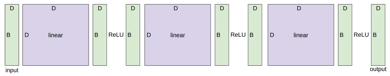
读图：deep network 图里的状态

每一层都有参数，forward 产生 activation，backward 需要 activation 和参数来计算 gradients。训练 memory 不是只有 parameters，还包括 gradients、optimizer state 和 activations。

对一层 \(h_2=h_1W_2\)，forward 约 \(2BD^2\) FLOPs。Backward 需要：

\[ \frac{\partial \ell}{\partial h_1} = \frac{\partial \ell}{\partial h_2}W_2^\top, \qquad \frac{\partial \ell}{\partial W_2} = h_1^\top\frac{\partial \ell}{\partial h_2}. \]

这两个矩阵乘法各约 \(2BD^2\)，所以 backward 是 forward 的约 2 倍。对总参数 \(P\)，训练一步粗估：

\[ \text{FLOPs per step}\approx 6BP. \]

6BP 公式的地位

这是大模型训练中最常用的粗账本之一。它忽略长上下文 attention 的额外项，但足以做训练时间数量级估计。

Optimizer state 与 training loop

状态	bytes/parameter	说明
Parameter	2	bf16 权重。
Gradient	2	bf16 梯度。
AdaGrad state	4	fp32 累积 squared gradients。
Adam state	8	fp32 first moment \(m\) + second moment \(v\)。

AdaGrad optimizer 的核心状态

g2 = state.get("g2", torch.zeros_like(grad))
g2 += torch.square(grad)
state["g2"] = g2
p.data -= lr * grad / torch.sqrt(g2 + 1e-5)

术语消化：SGD、Momentum、AdaGrad、RMSProp、Adam

SGD 只用当前梯度；Momentum 对梯度做指数平均；AdaGrad 用历史梯度平方缩放学习率；RMSProp 对梯度平方做指数平均；Adam 同时维护一阶动量 \(m\) 和二阶动量 \(v\)，因此状态显存较大但训练稳定。

最小训练循环

for step in range(num_train_steps):
    x, y = get_batch()
    pred_y = model(x).mean()
    loss = F.mse_loss(pred_y, y)
    loss.backward()
    optimizer.step()
    optimizer.zero_grad(set_to_none=True)

zero grad 不是细节

PyTorch 默认会累积 gradients。不清零会把上一步的梯度混入下一步。set_to_none=True 还能减少不必要的显存写入。

本章小结

训练一步可以拆成 forward、backward、optimizer step。Backward 通常约为 forward 的 2 倍；Adam 的 optimizer state 可能比参数本身更占显存；activations 则随 batch、sequence、layers 增长。

Memory Optimization：用资源交换资源

Gradient accumulation

大 batch 提高训练稳定性，但 activation memory 随 batch 增长。Gradient accumulation 把 global batch 切成多个 micro-batches，每个 micro-batch 计算梯度并累积，累积够再 step。

\[ \text{micro batch size}=\frac{\text{global batch size}}{\text{accumulation steps}}. \]

Gradient accumulation 的 tradeoff

它降低每次 forward/backward 的 activation 峰值，但不会减少总 FLOPs；代价是一次参数更新前要跑多个 micro-batches。

Activation checkpointing

Activation checkpointing 也叫 gradient checkpointing 或 rematerialization。它不是“把模型权重保存到磁盘”的 model checkpointing，而是 forward 时只保存部分 activations；backward 需要未保存的 activation 时，从最近 checkpoint 重新计算一段 forward。

读图：同一张 deep network 图的第二种读法

前面这张图用于计算 forward/backward FLOPs；这里它用于追踪 activation 生命周期。若保存每层输出，显存是 \(O(L)\)；若只保存检查点，中间 activation 可以重算，从而用更多 compute 换更少 memory。

策略	activation memory	compute overhead
存所有层	\(O(L)\)	无额外重算。
不存中间层	\(O(1)\)	可能 \(O(L^2)\)，每层 backward 前从头重算。
每 \( L\) 层存 checkpoint	\(O( L)\)	\(O(L)\) 级别重算，常见折中。

内存优化不是免费午餐

Gradient accumulation 用更多 micro-step 换更低 activation 峰值；activation checkpointing 用重算换显存；ZeRO/FSDP 用通信换显存。所有技巧都是资源交换，必须放回整体训练时间和稳定性中判断。

端到端训练前 checklist

检查项	手算方法	失败信号
参数量	逐层数矩阵大小，或粗估 \(P\)	参数相关显存已超设备容量。
训练 FLOPs	\(C≈ 6P D_tokens\)	训练时间远超预算。
参数/梯度/优化器显存	bf16 参数 2B、梯度 2B、Adam state 8B/param	不算 activation 都放不下。
Activation memory	粗估 \(O(BSLD)\) 或 profiler 外推	batch/context 一大就 OOM。
Arithmetic intensity	FLOPs / bytes moved	太低说明 kernel 可能 memory-bound。
MFU	actual FLOP/s / promised FLOP/s	远低于 0.5 需要检查 kernel、通信和数据加载。

本章小结

Memory optimization 的核心是 tradeoff。没有一种技巧单独解决所有问题；实际大模型训练往往组合 gradient accumulation、checkpointing、ZeRO/FSDP、tensor/pipeline parallelism 和 kernel fusion。

补充推导：把本讲公式真正用起来

从 dtype 到显存：三个数量级例子

下面三个例子把 dtype 账本落到真实 LLM 场景。

对象	估算	含义
单个 GPT-3 FFN 矩阵	\(12288× 4· 12288\) 个参数，bf16 约 1.2GB，fp32 约 2.4GB	单层矩阵已经是 GB 级，不能把权重读写当成免费。
70B bf16 参数	\(70B× 2≈ 140\)GB	只存参数就超过单张 80GB H100。
70B AdamW 状态	参数 140GB + 梯度 140GB + Adam state 560GB	不 sharding 时，训练状态远大于参数本身。

为什么 optimizer state 经常比模型更吓人

很多人第一次估算显存只算参数，这是错误的。AdamW 的两个 fp32 state 各自和参数数量一样大：\(m\) 记录梯度方向的一阶指数平均，\(v\) 记录梯度平方的二阶指数平均。若参数是 bf16，两个 fp32 state 合计是参数显存的 4 倍。

Einops worked examples：维度如何决定算子语义

einsum 明确说明 contracting dimension

# x: [batch, seq1, hidden]
# y: [batch, seq2, hidden]
# hidden appears on the left but not the right, so it is summed over.
z = einsum(x, y, "batch seq1 hidden, batch seq2 hidden -> batch seq1 seq2")

rearrange 把一个维度拆成 heads 和 hidden

# x: [seq, total_hidden], total_hidden = heads * hidden1
x = rearrange(x, "seq (heads hidden1) -> seq heads hidden1", heads=2)
x = einsum(x, w, "seq heads hidden1, hidden1 hidden2 -> seq heads hidden2")
x = rearrange(x, "seq heads hidden2 -> seq (heads hidden2)")

Einops 不是语法糖这么简单

命名维度让你在写代码时显式声明哪些维度被求和、哪些维度被保留、哪些维度被拆分。这正是后续 attention、tensor parallelism、sequence parallelism 的语言。

Arithmetic intensity worked examples

对 bf16 ReLU，读 \(x\) 和写 \(y\) 各 2 bytes，计算约 1 FLOP/element：

\[ I_{\mathrm{ReLU}}\approx \frac{n}{4n}=0.25\ \text{FLOPs/byte}. \]

对 bf16 matrix-vector product，\(x\in\mathbb{R}^n\)、\(W\in\mathbb{R}^{n\times n}\)：

\[ I_{\mathrm{matvec}} \approx \frac{2n^2}{2n^2+4n} \approx 1. \]

对 bf16 matrix-matrix multiplication，\(X,W\in\mathbb{R}^{n\times n}\)：

\[ I_{\mathrm{matmul}} \approx \frac{2n^3}{6n^2} =\frac{n}{3}. \]

为什么 matmul 是训练的朋友，matvec 是推理的麻烦

Matrix-matrix 让同一块权重被许多 batch/sequence 位置复用，\(I\) 随 \(n\) 增长；matrix-vector 每次只服务少量 token，读完整权重却复用很少。这就是训练 prefill 容易 compute-bound，而 autoregressive decode 容易 memory-bound 的根源。

训练状态生命周期图

阶段	状态变化
Get batch	data 从 CPU/dataloader 进入 GPU。
Forward	读取 parameters，写 activations，产生 logits/loss。
Backward	读取 activations 和 parameters，写 gradients；部分 activations 可逐层释放。
Optimizer step	读取 gradients 和 optimizer state，更新 parameters、\(m\)、\(v\)。
Zero grad	清理 gradients，准备下一步；若不清理会累积。

生命周期比总量更重要

峰值显存取决于哪些 tensor 同时存在。Parameters 和 optimizer state 常驻；activations 在 backward 中逐渐释放；temporary buffers 只在 kernel 调用期间存在。Profiler 看到的是生命周期重叠后的峰值，而不是简单加总。

ZeRO、checkpointing、accumulation 如何组合

技术	主要省什么	主要代价
Gradient accumulation	降低每个 micro-batch 的 activation 峰值	多次 forward/backward 才更新一次参数。
Activation checkpointing	少存中间 activations	backward 时重算 forward 片段。
ZeRO-1	optimizer state	optimizer step 需要跨卡协调。
ZeRO-2	optimizer state + gradients	梯度 reduce-scatter 等通信增加。
ZeRO-3	optimizer state + gradients + parameters	forward/backward 前后需要 all-gather 参数，通信更多。

不要把 ZeRO 当成 tensor parallelism

ZeRO 是 data parallel 框架里的状态分片技术，核心是减少重复存储；tensor parallelism 是把单层矩阵计算切到多卡上，核心是拆计算。两者经常组合，但解决的问题不同。

逐节点补充：源码中的资源核算细节

motivating questions 的完整推导

第一个问题“70B on 15T tokens on 1024 H100s”可以拆成三层：模型计算量、硬件有效速度、训练天数。

\[ C = 6ND = 6\times 70\times 10^9\times 15\times 10^{12}=6.3\times 10^{24}. \]

H100 dense bf16 峰值按 \(1979/2\) TFLOP/s 估算，乘以 MFU 0.5 和 1024 张卡：

\[ \text{effective FLOP/s}=1024\times 0.5\times 989.5\times 10^{12}. \]

训练天数为：

\[ \frac{6.3\times 10^{24}}{1024\times 0.5\times 989.5\times 10^{12}\times 86400}\approx 144\text{ days}. \]

这个 144 天不是承诺排期

它没有算 dataloader、checkpoint、通信、故障恢复、验证、warmup、重启、调参和集群排队。它只是告诉你：这个训练不是“几天跑完”的量级，必须靠 scaling law 和小实验减少盲试。

第二个问题“8 H100 using AdamW 最大模型”同样要拆开：

状态	每参数字节	说明
参数	2	bf16 参数。
梯度	2	训练时 backward 产生，常用 bf16。
Adam 一阶动量	4	fp32 \(m\)。
Adam 二阶动量	4	fp32 \(v\)。

总计 12 bytes/parameter。8 张 80GB H100 总共 640GB，除以 12 得到约 53B 参数。但这只是参数相关状态，不含 activations，所以真实可训练规模更小。

dtype 数值范围为什么影响训练稳定性

fp16 的问题不是“精度少一点”这么简单，而是 exponent 位数少导致动态范围窄。比如 \(10^{-8}\) 这类小数可能在 fp16 下直接 underflow 成 0；如果梯度或 optimizer 统计出现类似情况，训练会不稳定。bf16 牺牲 mantissa 精度，保留 fp32 的 exponent 宽度，所以更适合大模型训练。

AMP 的实用直觉

Automatic Mixed Precision 并不是把所有操作都换成低精度。矩阵乘法、卷积等通常能安全使用 bf16/fp16；softmax、exp、optimizer state、某些 reduction 更需要高精度。AMP 的价值是把这些选择自动化，但理解背后的 dtype 账本仍然重要。

FLOPs 计数里的“乘加各一次”

矩阵乘法 \(Y=XW\)，输出元素为：

\[ Y_{ik}=\sum_{j=1}^{D}X_{ij}W_{jk}. \]

对每个 \((i,k)\)，需要 \(D\) 次乘法和约 \(D\) 次加法，所以近似 \(2D\) FLOPs。输出共有 \(B\times K\) 个元素，因此：

\[ \mathrm{FLOPs}(XW)\approx 2BDK. \]

为什么 FLOPs 计数要保留近似意识

严格说加法是 \(D-1\) 次，不是 \(D\) 次；但大模型资源估算关注数量级，\(2BDK\) 的近似足够好。真正危险的是漏掉 backward 或 optimizer state，而不是纠结 \(-1\) 项。

从 arithmetic intensity 到 kernel 优化策略

如果一个操作 memory-bound，提高 peak FLOP/s 不一定有帮助，因为计算单元在等数据。常见优化方向是：

• fusion：把多个小 kernel 合并，减少中间结果写回 HBM。
• tiling：让数据块进入 SRAM/cache 后被多次复用。
• layout change：改变 tensor 排布，让访问连续、coalesced。
• batching：增大矩阵维度，提高权重复用。

first-use glossary：HBM、SRAM 和 fusion

HBM 是 High Bandwidth Memory，GPU 上的大容量高带宽显存；SRAM 是 Static Random-Access Memory，通常指芯片内部更小但更快的片上存储/cache。Fused kernel 的目标是让数据从 HBM 读入后，在片上连续完成多个操作，最后只写回一次，从而减少 HBM 往返。

Activation checkpointing 与 model checkpointing 的区别

这两个词都叫 checkpoint，但意思完全不同：

术语	保存什么	目的
Model checkpointing	参数、optimizer state、训练步数等写到磁盘	故障恢复、保存模型版本。
Activation checkpointing	forward 中只保存部分中间 activations	用重算换显存，支持更深模型/更大 batch。

不要把两种 checkpoint 混为一谈

Model checkpointing 面向训练任务生命周期；activation checkpointing 面向单次 forward/backward 内部的显存峰值。前者通常增加 I/O，后者通常增加 compute。

总结与延伸

Lecture 2 建立了大模型训练的最小资源语言：

1. Tensor 是 data、parameters、gradients、optimizer state、activations 的统一载体。
2. Memory 由 numel、dtype、device 和生命周期决定。
3. FLOPs 是计算量，FLOP/s 是速度，MFU 衡量有效硬件利用率。
4. Arithmetic intensity 判断 memory-bound 和 compute-bound。
5. 训练一步常用 \(6BP\) 粗估，但 memory 还要算 optimizer state 和 activations。
6. Gradient accumulation、activation checkpointing、ZeRO/FSDP 都是资源交换。

最终 takeaway

Resource accounting 是 CS336 的工程底座。不会算 FLOPs、memory 和 bandwidth，就无法判断一个训练 recipe 是否可行，也无法理解后续 kernels、parallelism、inference 和 scaling laws 为什么这样设计。

拓展阅读

• JAX Scaling Book: roofline and systems chapters.
• NVIDIA H100/B200 datasheets and Transformer Engine FP8 documentation.
• PyTorch AMP, activation checkpointing, and optimizer documentation.
• Transformer memory and FLOPs accounting blog posts.